Vulnerability, Exposure, and Impacts


Lecture

Mon., Jan. 22

Today

Given some hazard, how do we assess the damages or impacts?

We can quantify this, for example as \[ \textrm{Damage} = \textrm{Vulnerability} \times \textrm{Exposure} \times \textrm{Hazard} \]

Let’s understand these terms through some examples!

Illustrative examples

Today

  1. Illustrative examples

  2. How to manage exposure and vulnerability?

  3. Some math

  4. Wrapup

Structural fragility curve

\[ \Pr(\textrm{failure}) = f(\textrm{hazard}, \theta) \]

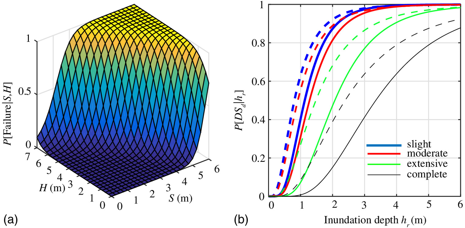
Figure 1: Parameterized fragilities as a function of surge and wave height for MSSS concrete bridges in South Carolina (a). (b): fragility curves for bridges subjected to tsunami hazard for low (solid lines) and moderate (dashed lines) flow rates (Gidaris et al., 2017).

Flood depth-damage curve

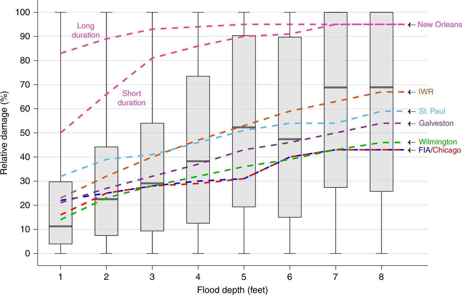
Figure 2: Boxplots show Wing et al. (2020) analysis of insurance claims. Lines show USACE depth-damage curves.

Seawall cost-benefit analysis

For a given storm, the total damages can be estimated by summing the damages for each property. \[ \textrm{Total damages} = \sum_{i \in \, \textrm{exposure}} \textrm{Hazard}_i \times \textrm{Vulnerability}_i \]

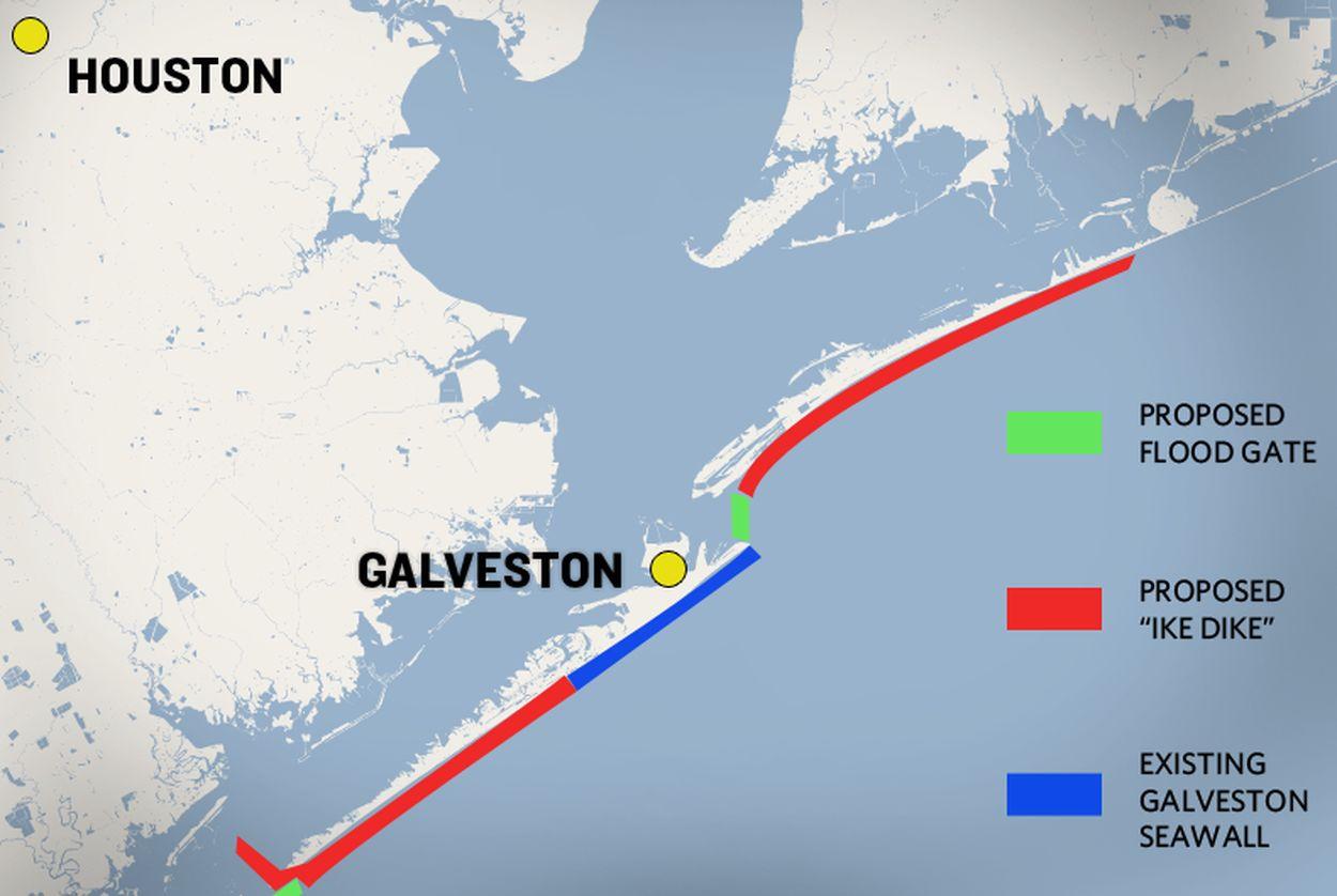
Figure 3: Proposed “Ike Dike”

Insurance portfolio risk

This is the most straightforward example of the exposure-vulnerability-hazard framework

  • Hazard: a real or synthetic storm
  • Exposure: all the assets that are insured
  • Vulnerability: predicted losses as a function of the hazard

How to manage exposure and vulnerability?

Today

  1. Illustrative examples

  2. How to manage exposure and vulnerability?

  3. Some math

  4. Wrapup

Trends in exposure

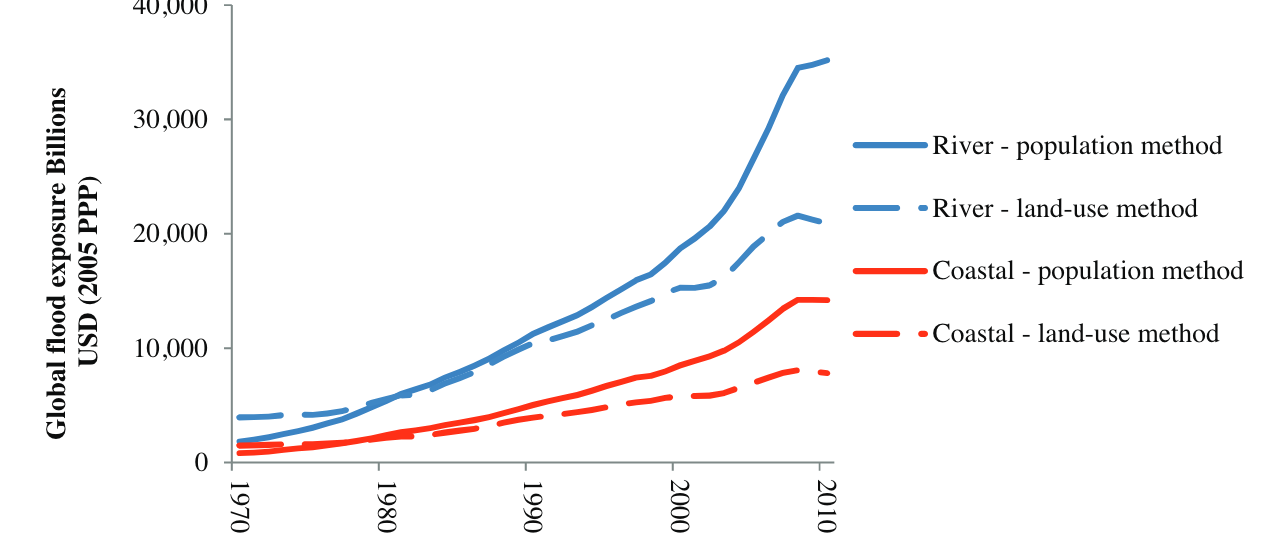
Figure 4: Global asset exposure to river and coastal flooding using the population and land-use methods (Jongman et al., 2012).

Example: North Carolina

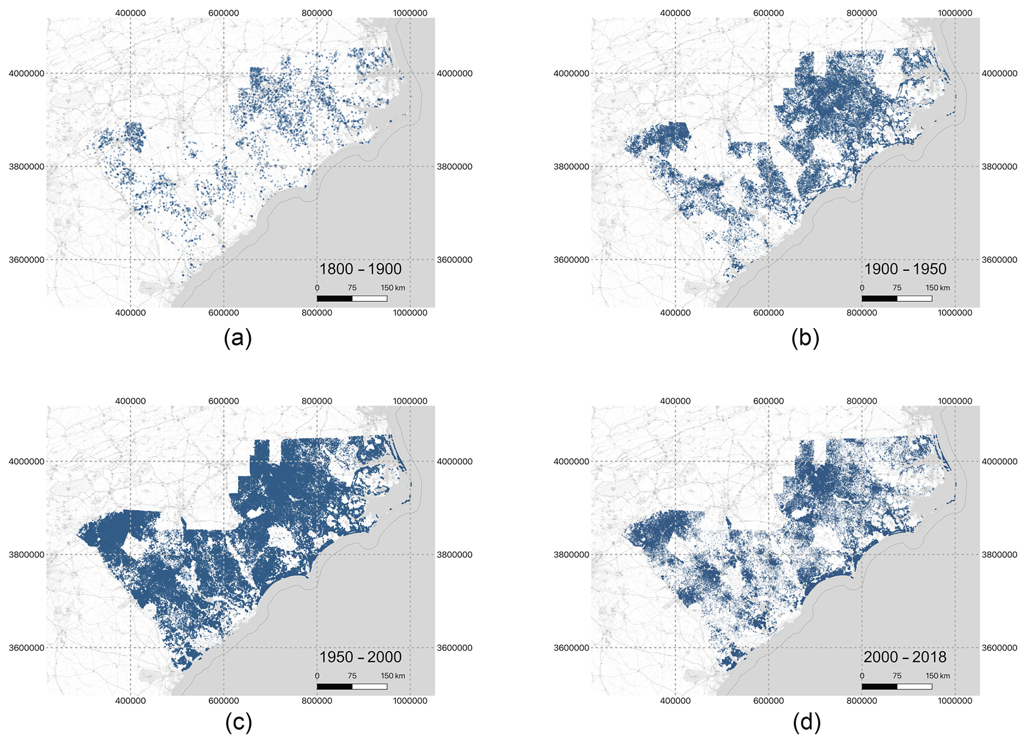
Figure 5: Spatial distribution of the properties within our database that were built during the (a) 1800–1900, (b) 1900–1950, (c) 1950–2000 and (d) 2000–2018 periods (Tedesco et al., 2020).

Changing vulnerability

Interventions such as floodproofing can shift the vulnerability curve

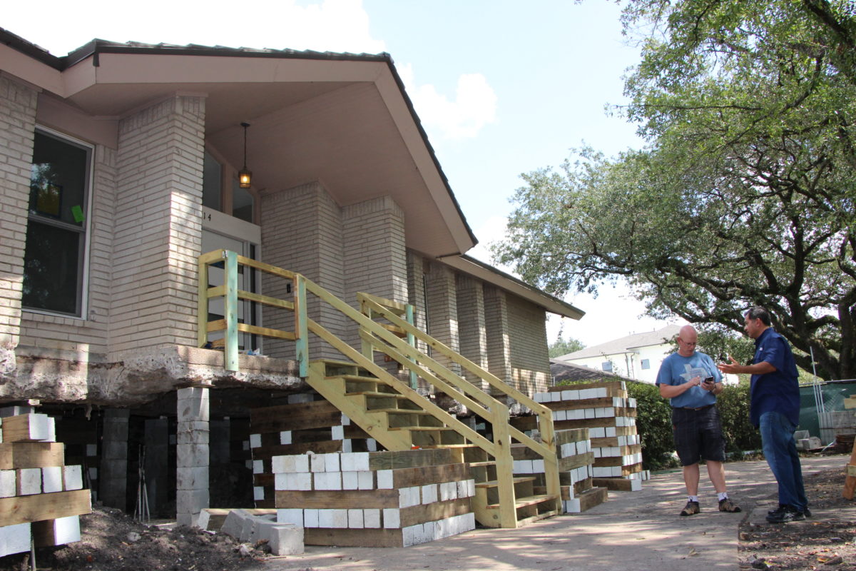
Figure 6: Floodproofing in Houston, TX (Houston Public Media)

Some math

Today

  1. Illustrative examples

  2. How to manage exposure and vulnerability?

  3. Some math

  4. Wrapup

Expectation

The expected value of a function \(f(x)\) of a random variable \(x\) is: \[ \mathbb{E}[f(x)] = \int f(x) p(x) dx \] where \(p(x)\) is the probability density function of \(x\).

In other words, for each possible value of \(x\), calculate \(f(x)\). We then take a weighted average, where the weights are the probability of each value of \(x\).

Key insight

You cannot get the expected value of a function by plugging the expected value of the random variable into the function. \[ \mathbb{E}[f(x)] \neq f(\mathbb{E}[x]) \]

Expected damages

If we want to calculate the expected damages then we can use this formula \[ \mathbb{E}[f(x)] = \int f(x) p(x) dx \] by defining \(x\) to be the hazard (e.g., flood depth) and \(f(x)\) the damage function.

Important

The key assumption we need is that we know the probability density function \(p(x)\)!

Monte Carlo approximation

In general, \(\int f(x) p(x) dx\) is hard to compute analytically. We can use Monte Carlo methods to approximate this integral.

Important

Monte Carlo methods are a wide class of computational algorithms for approximating integrals.

Monte Carlo expectation

If we draw \(N\) samples independently and identically distributed (i.i.d.) from a probability distribution \(p(x)\), denoted as \(\left\{x_i\right\}_{i=1}^N\) where \(x_i \sim p(x)\), then \[ \mathbb{E}[f(x)] \approx \frac{1}{N} \sum_{i=1}^N f(x_i) \]

Tip

Drawing \(N\) samples iid from \(p(x)\) can be inefficient. Most of the samples will be in regions where \(f(x)\) is small, so we are wasting computational effort. There are many clever ways around this.

For example: Trapezoidal EAD

Running regional flood models is computationally expensive. Often, a model may have been run for a few different nominal return levels. For example, we might have flood depths at each grid for the nominal 10, 25, 50, 100, 250, and 500 year floods.

Figure 7: Moel et al. (2014) uses trapezoidal methods to approximate the expected annual damages.

Wrapup

Today

  1. Illustrative examples

  2. How to manage exposure and vulnerability?

  3. Some math

  4. Wrapup

Key points

  1. Impacts (damage) depend on hazard, exposure, and vulnerability.
  2. Exposure and vulnerability are changing rapidly.
  3. To estimate risk, we need a model for how our system responds to a hazard.
  4. If we know the probability density function of the hazard, we can use Monte Carlo methods to estimate expected impacts.

Limitations of this framework

  1. How to think about damages that are not direct damages (e.g., “indirect” damages)?
  2. How to think about complex systems and risks (e.g., breadbasket failures) that are not easy summarized by a single metric?

Logistics

  • Wednesday: discussion questions for Wing et al. (2020) posted
  • Wednesday after class: troubleshoot computing issues
  • Friday: lab
Gidaris, I., Padgett, J. E., Barbosa, A. R., Chen, S., Cox, D., Webb, B., & Cerato, A. (2017). Multiple-Hazard Fragility and Restoration Models of Highway Bridges for Regional Risk and Resilience Assessment in the United States: State-of-the-Art Review. Journal of Structural Engineering, 143(3), 04016188. https://doi.org/10.1061/(ASCE)ST.1943-541X.0001672
Jongman, B., Ward, P. J., & Aerts, J. C. J. H. (2012). Global exposure to river and coastal flooding: Long term trends and changes. Global Environmental Change, 22(4), 823–835. https://doi.org/10.1016/j.gloenvcha.2012.07.004
Moel, H. de, Vliet, M. van, & Aerts, J. C. J. H. (2014). Evaluating the effect of flood damage-reducing measures: A case study of the unembanked area of Rotterdam, the Netherlands. Regional Environmental Change, 14(3), 895–908. https://doi.org/10.1007/s10113-013-0420-z
Tedesco, M., McAlpine, S., & Porter, J. R. (2020). Exposure of real estate properties to the 2018 Hurricane Florence flooding. Natural Hazards and Earth System Sciences, 20(3), 907–920. https://doi.org/10.5194/nhess-20-907-2020
Wing, O. E. J., Pinter, N., Bates, P. D., & Kousky, C. (2020). New insights into US flood vulnerability revealed from flood insurance big data. Nature Communications, 11(1, 1), 1444. https://doi.org/10.1038/s41467-020-15264-2