Policy Search and Optimization
Lecture
Mon., Feb. 19
Overview
Today
Overview
Optimization in the wild
Wrapup
Review of notation
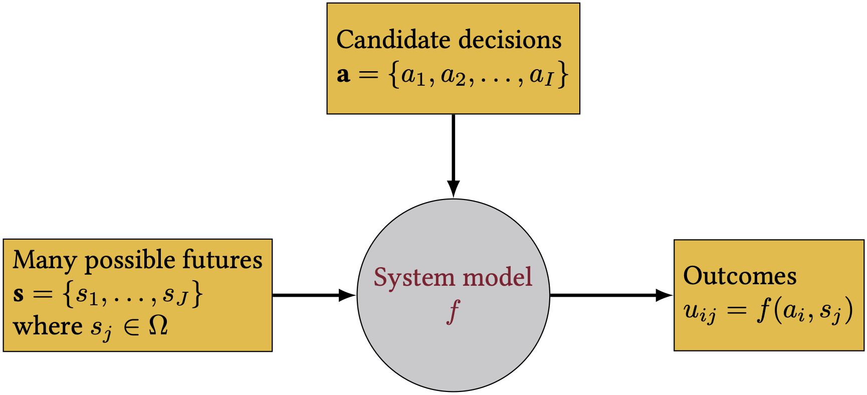
Figure 1: Notation for our system dynamics.
Key components of an optimization problem
- Objective function
- Constraints
- Decision variables
Reflect
To what extent is this [in]consistent with exploratory modeling?
Why optimize?
Large action spaces (many decision variables) make it difficult to find the best solution by trial and error.
Important
Today we’ll say optimization but even an exact solution is only optimal in our model, not the real world. I prefer the term policy search which emphasizes the use of computers to suggest promising strategies.
Optimization in the wild
Today
Overview
Optimization in the wild
Wrapup
Where have you seen optimization used?
Reflect
Take 2-3 minutes, then share.
Linear programming
Find a vector \(\mathbf{x}\) that maximizes \(c^T \mathbf{x}\) subject to \(A \mathbf{x} \leq \mathbf{b}\) and \(\mathbf{x} \geq 0\) (Wikipiedia)
- Limitations: requires strong assumptions (is linearizing your function a good approximation?)
- Strengths: very fast (can scale to large problems)
- Examples: how much should each pump in a water distribution network be run at a given time step to maintain pressure?
Linear programming with discrete decisions
- Fixed costs create discontinuities in the objective function
- Example: which electricity generators should be on/off?
- Need to create new indicator variables which flag on/off status: \(\mathbb{I}_i = \begin{cases} 0 & \textrm{off} \\ 1 & \textrm{on} \end{cases}\).
- Can be solved with mixed-integer linear programming (MILP)
Gradient descent
If you have a differentiable function, you can use gradient descent to find the minimum.
\[ \mathbf{x}_{n+1} = \mathbf{x}_n - \alpha \nabla f(\mathbf{x}_n) \]
See illustration here

Simulation-optimization
- Strengths: can handle complex, non-linear systems (model can be a black box)
- Limitations: slow (“guess and check”), rely on “heuristics” to decide a solution is good enough
- Examples: design of water resource systems under uncertainty
Tip
We’ll use simulation-optimization in our lab next week.
Wrapup
Today
Overview
Optimization in the wild
Wrapup
Key points
- Optimization can be used at a high level (e.g., system design) or can be embedded in a problem (e.g., operations at each time step).
- Every optimization problem has an objective and decision variables. Many have constraints.
- Optimization is a field, with many techniques.
- In this course, I want you to understand and critique how optimization problems are framed in the wild. Take other courses to focus on the techniques.
Wednesday
We will discuss @Schwetschenau et al. (2023). Discussion questions are posted. Please focus on the framing of the problem and the assumptions made when you read; don’t get bogged down in the technical details.
Learn more
References
Schwetschenau, S. E., Kovankaya, Y., Elliott, M. A., Allaire, M., White, K. D., & Lall, U. (2023). Optimizing Scale for Decentralized Wastewater Treatment: A Tool to Address Failing Wastewater Infrastructure in the United States. ACS ES&T Engineering, 3(1), 1–14. https://doi.org/10.1021/acsestengg.2c00188