Genetic / algorithms are not exact methods. They rely on heuristics to decide a solution is “good enough” even if it’s not a global optimum. However, we can and should test our solutions for convergence and quality.
Repeat the optimization with different initial conditions (“random seeds”). Do results change?
Use diagnostics like hypervolume to measure how much of the Pareto front we’ve found.
Compare to other methods (e.g., weighted sum) to see if we’re missing parts of the Pareto front.
Compare solutions to human-generated benchmarks.
Wrapup
Today
Motivation
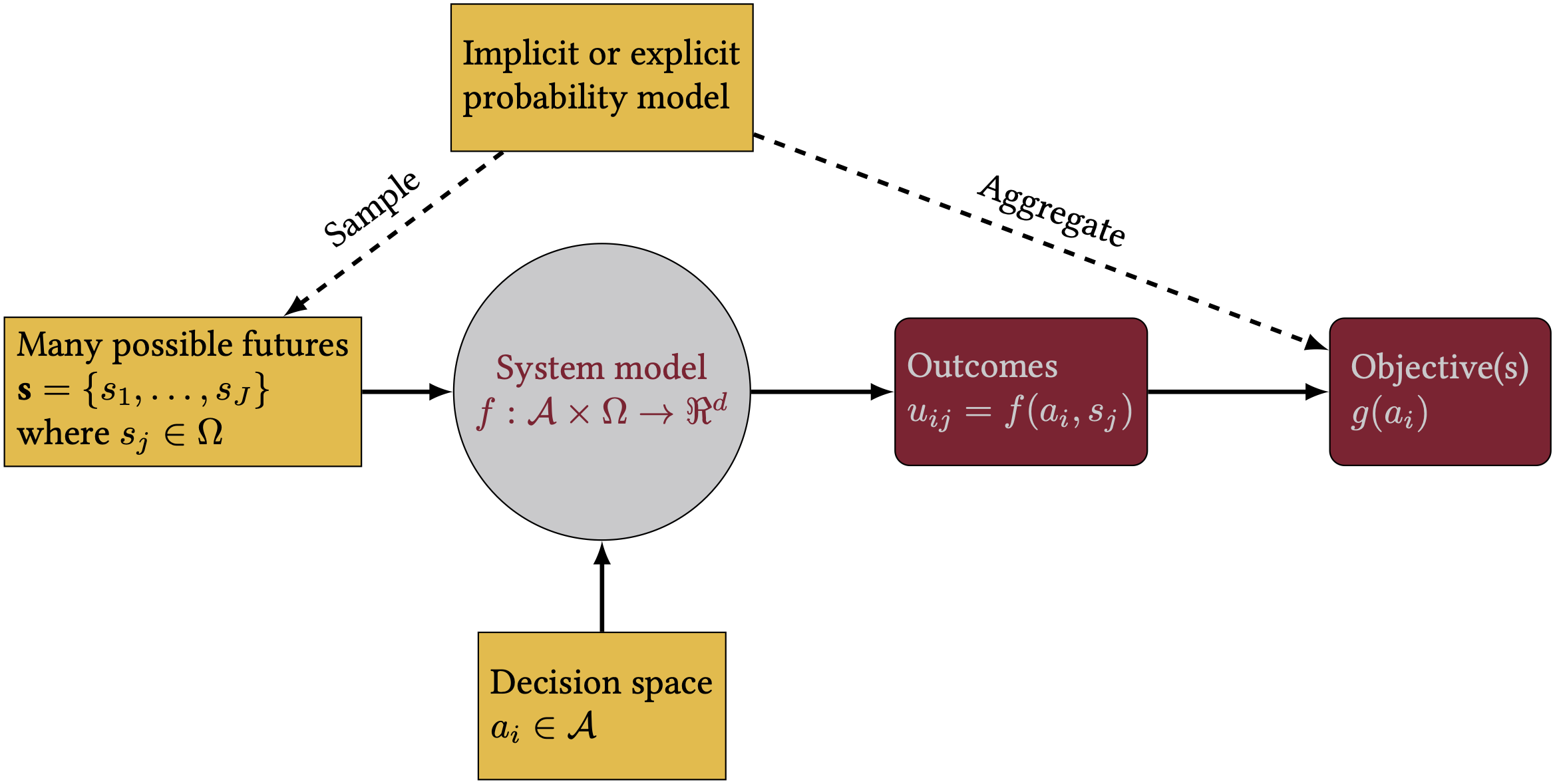
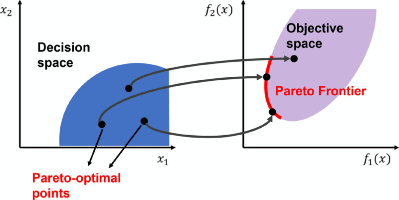
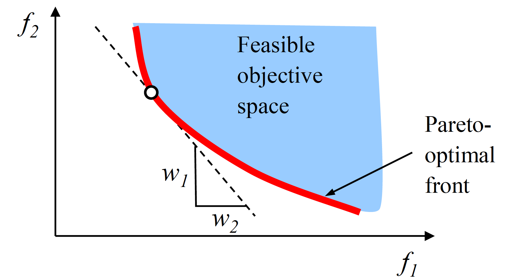
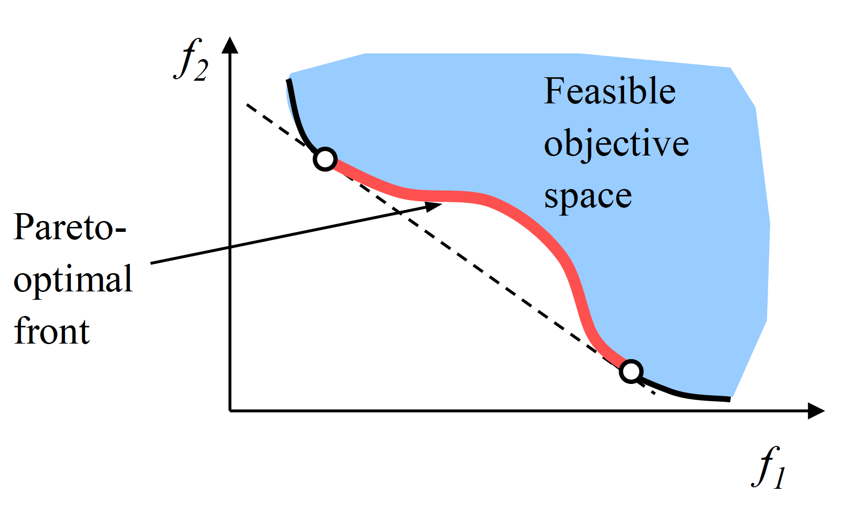
Multiobjective optimization
Implementation
Wrapup
Key ideas
Policy search
Multiobjective optimization
Genetic algorithms
How many objectives do we need?
There are drawbacks to adding more objectives:
Computational cost (exponentially more solutions needed)
Conceptual complexity
Difficulty communicating results
so we want as few as possible. Thus, combining objectives into a single function is often a good idea, when appropriate.
Kasprzyk, J. R., Nataraj, S., Reed, P. M., & Lempert, R. J. (2013). Many objective robust decision making for complex environmental systems undergoing change. Environmental Modelling & Software, 42, 55–71. https://doi.org/10.1016/j.envsoft.2012.12.007
Smith, S., Southerby, M., Setiniyaz, S., Apsimon, R., & Burt, G. (2022). Multiobjective optimization and Pareto front visualization techniques applied to normal conducting rf accelerating structures. Physical Review Accelerators and Beams, 25(6), 062002. https://doi.org/10.1103/PhysRevAccelBeams.25.062002
Zarekarizi, M., Srikrishnan, V., & Keller, K. (2020). Neglecting uncertainties biases house-elevation decisions to manage riverine flood risks. Nature Communications, 11(1, 1), 5361. https://doi.org/10.1038/s41467-020-19188-9