Hazard, Exposure, Vulnerability

Lecture

Dr. James Doss-Gollin

Wednesday, January 21, 2026

What Is a Fair Insurance Premium?

Target: 1:00. Open with a question that motivates the math.

You own a house in a flood zone.

An insurance company offers you a policy.

How do they decide what to charge you?

Today: The math behind flood risk pricing.

Quick Estimate

Target: 1:03. Get brains working immediately. Give 30 seconds to think, then cold call 2-3 students.

A house faces two possible flood scenarios this year:

Scenario	Probability	Damage
No flood	80%	$0
3 ft flood	20%	$50,000

What’s the expected annual damage?

(30 seconds to think)

Quick Estimate: Answer

Target: 1:05. Key insight: we weight by probability.

\[E[\text{Damage}] = 0.8 \times \$0 + 0.2 \times \$50,000 = \$10,000\]

This simple calculation is the core of risk analysis.

Today: How do we do this when floods and damages are continuous?

Today

Target: 1:07. Quick roadmap.

1. Define key vocabulary: hazard, exposure, vulnerability
2. See how these combine to produce risk
3. Learn why \(E[f(x)] \neq f(E[x])\) (Jensen’s inequality)
4. Introduce Monte Carlo for complex damage functions

Risk Analysis Vocabulary

Today

1. Risk Analysis Vocabulary

2. From Components to Risk

3. Convolution: Hazard → Damages

4. Extreme Value Theory

5. The House Elevation Problem

6. Wrap Up

Hazard

Target: 1:10. Emphasize that hazard is the physical event, not the damage.

Hazard: The physical event or phenomenon

• Flood depth at a location
• Wind speed during a storm
• Ground shaking from an earthquake
• Extreme temperature

Key insight: Hazards are characterized by probability distributions, not single values.

Exposure: What’s at Risk?

Target: 1:12. Exposure is about WHAT is at risk, not how vulnerable it is.

Exposure = assets that could be affected

• Buildings and infrastructure
• People and livelihoods
• Agricultural land
• Economic activity

Figure 1: Global flood exposure has grown 10× since 1970. Source: (jongman_exposure:2012?)

Exposure Changes Over Time

Target: 1:14. Local example: Houston’s footprint has exploded.

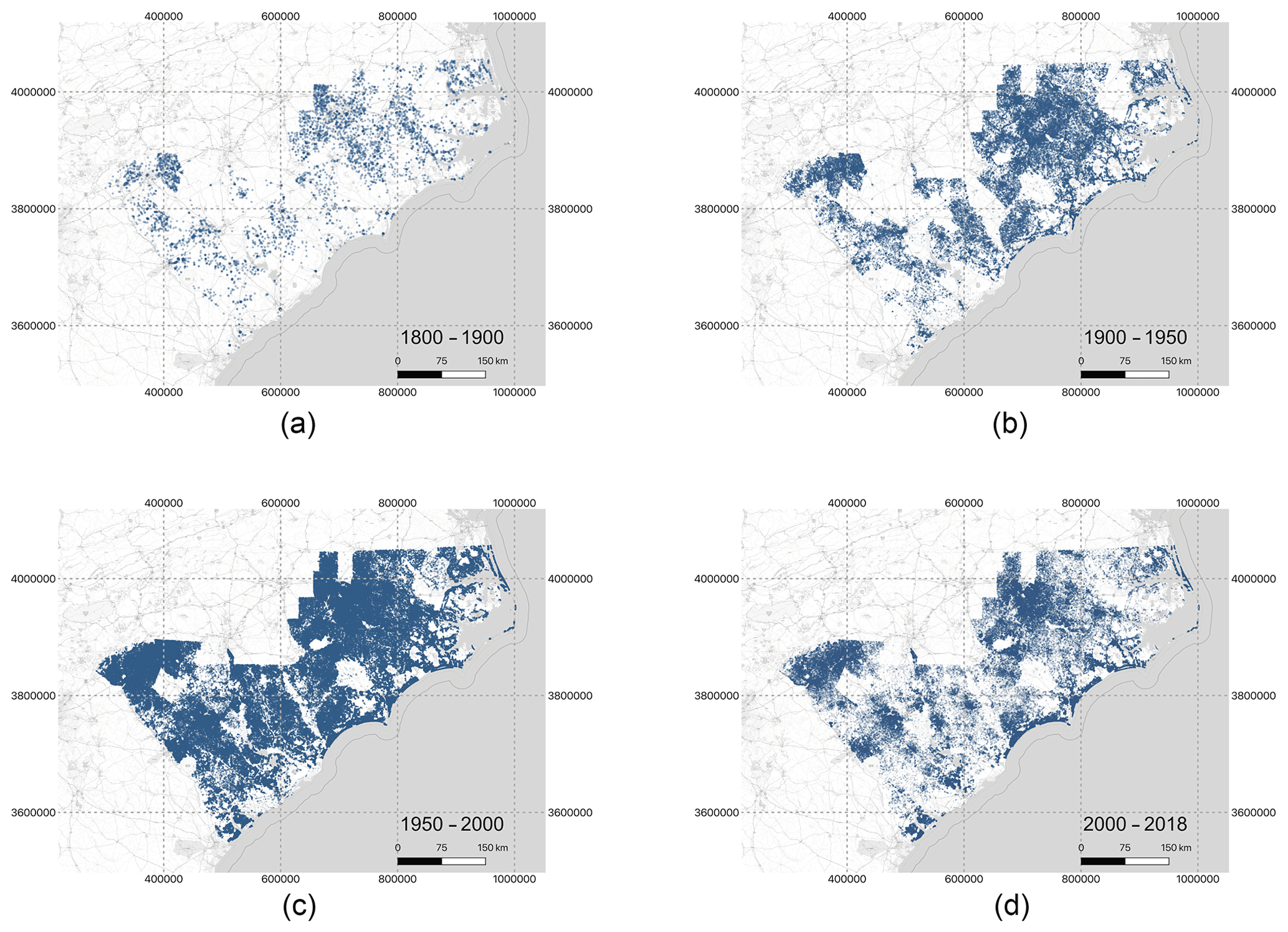
Figure 2: Houston’s built footprint 1800-2018. Development into flood-prone areas increases exposure. Source: (tedesco_exposure:2020?)

Vulnerability

Target: 1:16. This is where depth-damage functions come in.

Vulnerability: Propensity to suffer damage given exposure to hazard

Important distinction:

• Fragility: Probability of failure (binary)
• Vulnerability: Degree of damage (continuous, 0-1)

Fragility vs. Vulnerability

Target: 1:18. Show the Gidaris figure - panel (a) is a 3D fragility surface, panel (b) shows fragility curves.

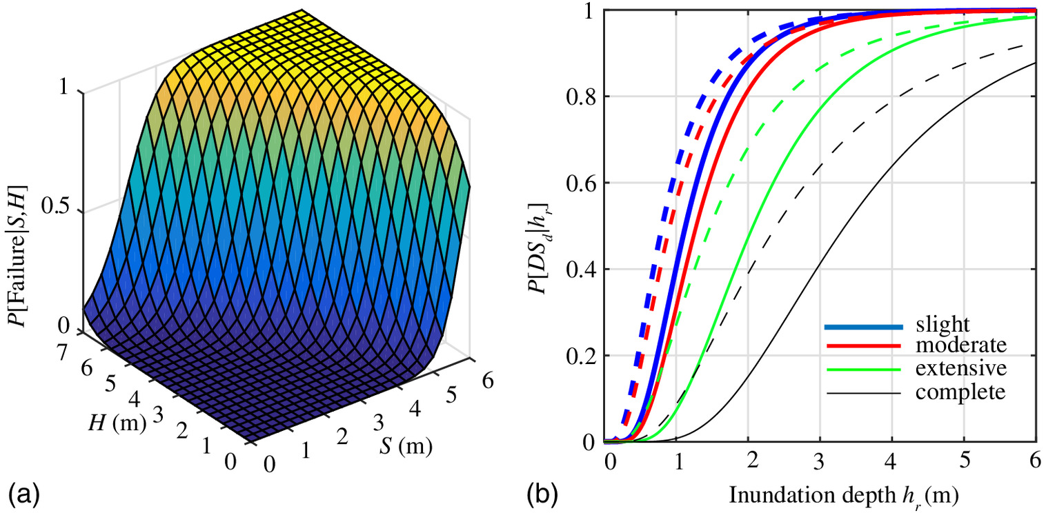
Figure 3: Fragility surfaces (a) and curves (b) show probability of damage given hazard intensity. Source: Gidaris et al. (2017)

Depth-Damage Functions

Target: 1:20. Show the Wing figure. Discuss the huge uncertainty in these relationships.

For floods, depth-damage functions quantify vulnerability:

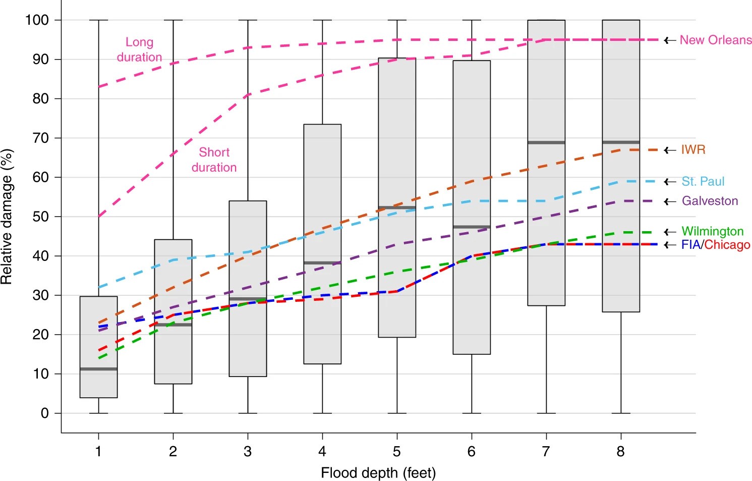
Figure 4: Empirical depth-damage from NFIP claims data. Boxplots: Wing et al. (2020) analysis. Lines: USACE engineering curves.

What Do You Notice?

Target: 1:22. Pause and ask students what they observe.

From the depth-damage data:

• Damage increases with depth (obvious)
• Huge uncertainty at any given depth
• Empirical data differs from engineering curves
• First foot of water causes significant damage

From Components to Risk

Today

1. Risk Analysis Vocabulary

2. From Components to Risk

3. Convolution: Hazard → Damages

4. Extreme Value Theory

5. The House Elevation Problem

6. Wrap Up

Risk = f(Hazard, Exposure, Vulnerability)

Target: 1:24. Core equation for the course. Write on board.

The fundamental equation:

\[\text{Damage} = \text{Vulnerability}(h) \times \text{Exposure}\]

where \(h\) is the hazard intensity (e.g., flood depth).

For expected damages, we integrate over the hazard distribution:

\[E[\text{Damage}] = \int \text{Vulnerability}(h) \times \text{Exposure} \times p(h) \, dh\]

Annual Expected Damages at Scale

Target: 1:26. This figure shows the full workflow from data to expected annual damage.

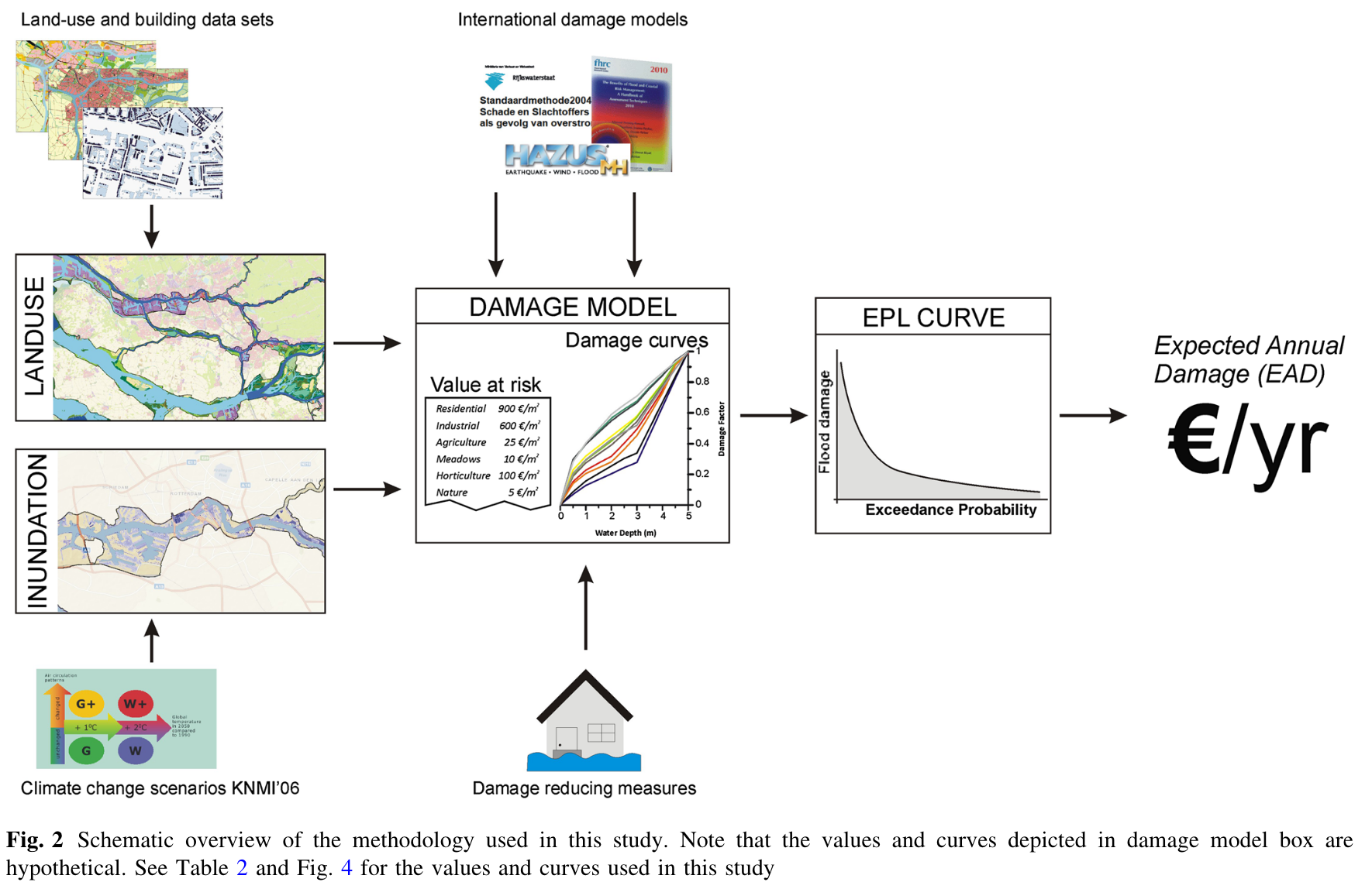
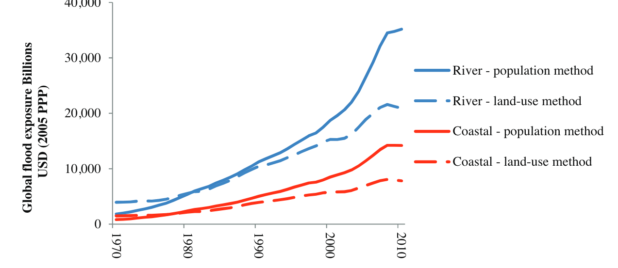
Figure 5: From hazard and exposure data through damage models to expected annual damage (EAD). Source: de Moel et al. (2014)

Your Turn

Target: 1:28. Give students 60 seconds to think. Then cold call 2-3 students.

A city is deciding whether to build a new seawall.

Identify the hazard, exposure, and vulnerability.

Discuss with a neighbor for 60 seconds.

Convolution: Hazard → Damages

Today

1. Risk Analysis Vocabulary

2. From Components to Risk

3. Convolution: Hazard → Damages

4. Extreme Value Theory

5. The House Elevation Problem

6. Wrap Up

The Key Mathematical Idea

Target: 1:32. This is the bridge to Friday’s lab. Draw on board if helpful.

We have:

• A hazard distribution \(p(h)\): probability of each flood depth
• A damage function \(D(h)\): damage given flood depth

We want:

• The damage distribution \(p(D)\): probability of each damage level

This transformation is called convolution.

Convolution Illustrated

Target: 1:34. Simple example to build intuition.

Hazard Distribution

• 50% chance: no flood (h=0)
• 30% chance: minor flood (h=2ft)
• 20% chance: major flood (h=6ft)

Damage Function

• h=0 → $0 damage
• h=2ft → $10,000 damage
• h=6ft → $100,000 damage

Damage Distribution:

• 50% chance: $0
• 30% chance: $10,000
• 20% chance: $100,000

Expected damage = $0.5(0) + 0.3(10k) + 0.2(100k) = $23,000

Jensen’s Inequality

Target: 1:36. Critical conceptual point. This equation WILL be on assessments. Draw convex function with secant line above curve.

For any nonlinear function \(f\):

\[E[f(x)] \neq f(E[x])\]

This will be on assessments. Know it.

Jensen’s Inequality: Example

Target: 1:38. Concrete example demonstrating the inequality.

Hazard:

• 50% chance: 2 ft flood
• 50% chance: 8 ft flood
• \(E[h] = 5\) ft

Damage function:

• \(D(2) = \$5,000\)
• \(D(8) = \$90,000\)
• \(D(5) = \$20,000\)

\(D(E[h]) = D(5) = \$20,000\)

\(E[D(h)] = 0.5(\$5k) + 0.5(\$90k) = \$47,500\)

The difference matters: $27,500 underestimate.

Why Monte Carlo?

Target: 1:40. Connect Monte Carlo to the integration problem.

For continuous distributions, expected damage is an integral:

\[E[D] = \int D(h) \cdot p(h) \, dh\]

This integral is intractable for nontrivial damage functions or probability density functions.

Solution: Monte Carlo integration approximates it with samples.

The Law of Large Numbers

Target: 1:42. Keep it simple - just the intuition.

If we draw \(N\) samples \(h_1, h_2, \ldots, h_N\) from \(p(h)\):

\[\frac{1}{N} \sum_{i=1}^{N} D(h_i) \xrightarrow{N \to \infty} E[D]\]

The sample average converges to the true expected value.

More samples → better approximation

Monte Carlo Recipe

Target: 1:43. Procedural summary connecting to lab.

1. Sample \(N\) flood scenarios from hazard distribution
2. Apply damage function: compute \(D(h_i)\) for each
3. Summarize the damage samples

Once we have samples, we can compute any statistic:

• Mean (expected annual damage)
• Variance (how much does damage vary year-to-year?)
• Quantiles (what’s the 99th percentile damage?)

This is exactly what you’ll implement on Friday.

Extreme Value Theory

Today

1. Risk Analysis Vocabulary

2. From Components to Risk

3. Convolution: Hazard → Damages

4. Extreme Value Theory

5. The House Elevation Problem

6. Wrap Up

Why Extremes Matter

Target: 1:44. Just planting the seed here. Deeper coverage in Week 4.

Most flood damage comes from rare, extreme events.

The problem: Normal distributions underestimate extreme risks.

We need specialized tools for modeling the tails of distributions.

The GEV Distribution

Target: 1:45. Keep it light. Just enough to use in lab.

The Generalized Extreme Value (GEV) distribution is designed for annual maxima.

Three parameters:

• \(\mu\) (location): Where the distribution is centered
• \(\sigma\) (scale): How spread out it is
• \(\xi\) (shape): How heavy the tail is

\(\xi > 0\) means fat tails: extreme events are more likely than a normal distribution predicts.

GEV in Practice

Target: 1:46. Preview what they’ll do in lab.

In lab on Friday, you will:

1. Define a GEV distribution for storm surge
2. Sample thousands of possible flood scenarios
3. Pass each through a depth-damage function
4. Analyze the resulting damage distribution

This is uncertainty quantification in action.

The House Elevation Problem

Today

1. Risk Analysis Vocabulary

2. From Components to Risk

3. Convolution: Hazard → Damages

4. Extreme Value Theory

5. The House Elevation Problem

6. Wrap Up

A Concrete Decision

Target: 1:47. Set up the problem students will use all semester.

A homeowner faces a choice:

How high should I elevate my house?

Higher elevation = more upfront cost, but less future flood damage.

House elevation in Meyerland, Houston. Photo: Allison Lee / Houston Public Media

The Trade-off

Target: 1:48. Draw on board if helpful.

• Elevate 0 feet: No construction cost, high expected damages
• Elevate 14 feet: High construction cost, near-zero damages
• Somewhere in between: ???

Finding the optimal elevation requires:

1. A hazard model (GEV distribution for surge)
2. A damage model (depth-damage function)
3. A cost model (construction costs by elevation)

This Semester’s Sandbox

Target: 1:48. Connect to the iCOW model and SimOptDecisions.

We’ll use the house elevation problem throughout the course:

Week	Topic	What We Add
2	Hazard-Damage Convolution	Basic Monte Carlo
3-5	Risk Metrics	EAD, VaR, CVaR
6-8	Decision Analysis	Optimal static decisions
10-13	Deep Uncertainty	Robust optimization

Wrap Up

Today

1. Risk Analysis Vocabulary

2. From Components to Risk

3. Convolution: Hazard → Damages

4. Extreme Value Theory

5. The House Elevation Problem

6. Wrap Up

Key Takeaways

Target: 1:49. Summarize main points.

1. Risk emerges from the interaction of hazard, exposure, and vulnerability
2. Exposure is growing: More assets in harm’s way
3. Convolution transforms hazard distributions into damage distributions
4. Monte Carlo lets us handle complex, nonlinear systems
5. The house elevation problem gives us a concrete sandbox

Lab Preview: Friday

Target: 1:50. Connect to Friday’s lab.

On Friday, you will:

1. Define a GEV distribution for storm surge
2. Implement a depth-damage function
3. Use Monte Carlo to compute damage distributions
4. Extend to 100 houses at varying elevations
5. Begin using the SimOptDecisions.jl framework

References

Gidaris, I., Padgett, J. E., Barbosa, A. R., Chen, S., Cox, D., Webb, B., & Cerato, A. (2017). Multiple-Hazard Fragility and Restoration Models of Highway Bridges for Regional Risk and Resilience Assessment in the United States: State-of-the-Art Review. Journal of Structural Engineering, 143(3), 04016188. https://doi.org/10.1061/(ASCE)ST.1943-541X.0001672

de Moel, H., van Vliet, M., & Aerts, J. C. J. H. (2014). Evaluating the effect of flood damage-reducing measures: A case study of the unembanked area of Rotterdam, the Netherlands. Regional Environmental Change, 14(3), 895–908. https://doi.org/10.1007/s10113-013-0420-z

Wing, O. E. J., Pinter, N., Bates, P. D., & Kousky, C. (2020). New insights into US flood vulnerability revealed from flood insurance big data. Nature Communications, 11(1, 1), 1444. https://doi.org/10.1038/s41467-020-15264-2