Models always trade off realism for tractability — they answer questions and inform decisions, not provide a 1:1 map of the real world.
With no computers available, van Dantzig needed a closed-form solution — so every assumption was chosen to keep the math tractable.
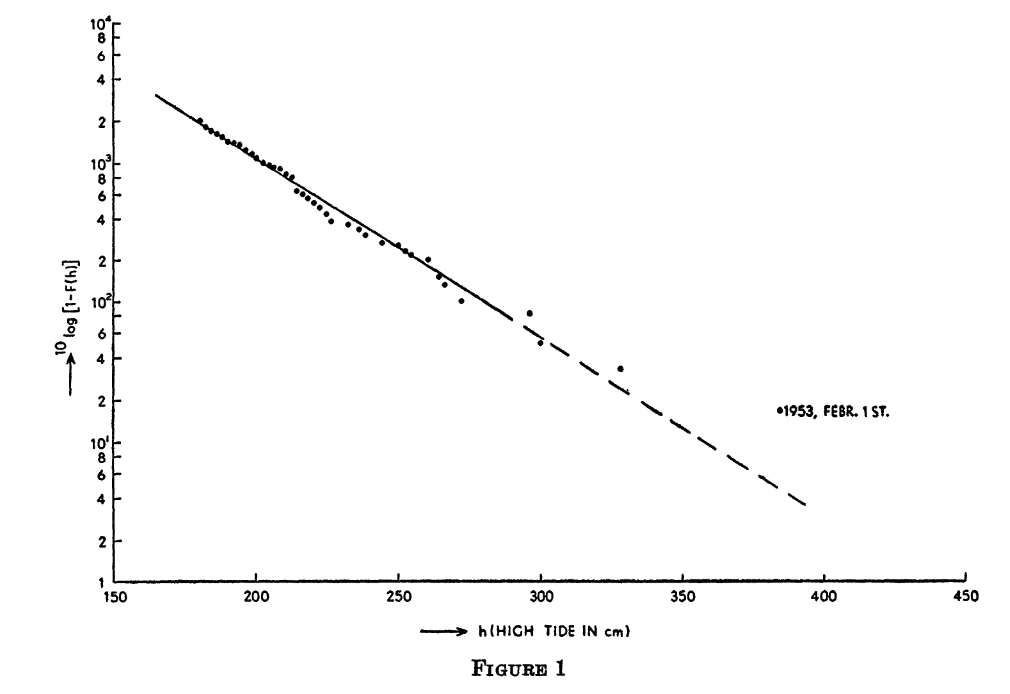
Flood Exceedance Probability
van Dantzig’s Figure 1: exceedance probability vs. high tide height at Hook of Holland. Note the 1953 event marked as an outlier. Source: van Dantzig (1956).
Assumed exponential exceedance probability:
\[
p(h) = p_0 \, e^{-\alpha(h - H_0)}
\]
\(h\) = water height
\(H_0\) = current dike height
\(p_0\) = current exceedance probability
\(\alpha\) = shape parameter
The straight line on the log plot is the exponential fit.
Why exponential? Because it makes the integral tractable.
The Loss Model
van Dantzig assumes binary damage: if water exceeds dike height \(H\), everything in the polder is lost.
\[
S = \begin{cases} 0 & \text{if } h \leq H \\ V & \text{if } h > H \end{cases}
\]
where \(V\) is the total value of all goods, buildings, farms, cattle, and industry in the polder.
Building the Cost Function
Construction cost (linear approximation): \[I(X) = I_0 + kX\]
Expected annual flood loss (probability \(\times\) total value at risk): \[p_0 \cdot V \cdot e^{-\alpha X}\]
Present value of ALL future expected losses (discounting!): \[L(X) = \frac{100 \, p_0 \, V \, e^{-\alpha X}}{\delta}\]
where \(\delta\) is the interest rate (in percent) — this is NPV, just like Week 5.
Figure 2: The classic trade-off: construction costs rise with dike height, expected losses fall. The optimum balances them. How would the optimum shift if the curves changed shape?
Optimal height increases when flood probability \(p_0\) is high
Optimal height decreases when discount rate \(\delta\) is high
Optimal height decreases when construction cost \(k\) is high
Adding Realism
Today
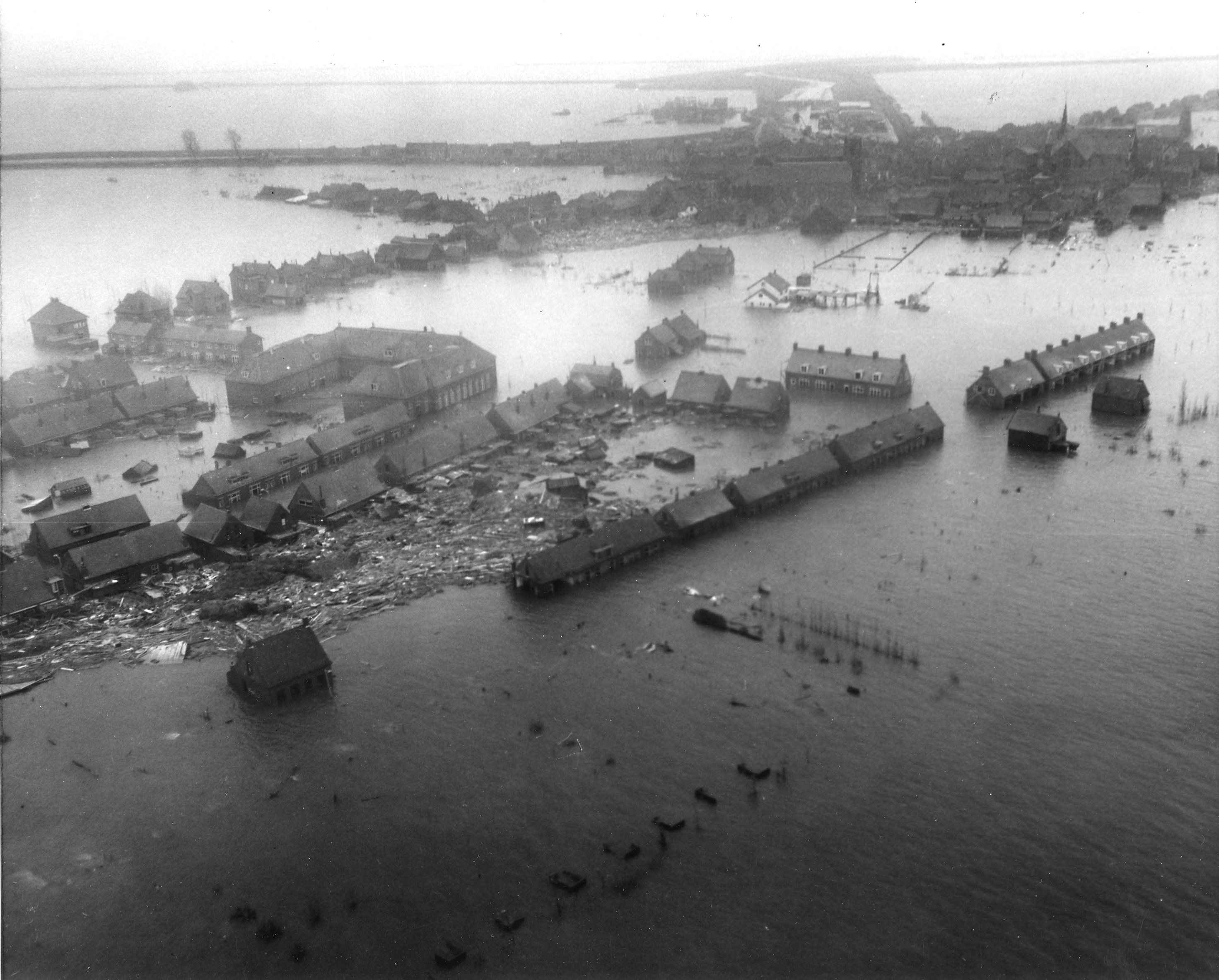
The 1953 North Sea Flood
van Dantzig’s Simple Model
Adding Realism
Optimization and Policy Search
Evaluating Optimization Claims
The Netherlands is Changing
Two slow processes push the optimal dike height higher:
Wealth growth: the economy grows at rate \(\gamma\) (estimated 1.5–2.5% per year), so \(V\) increases over time.
Land subsidence: the Netherlands has been sinking for 9,000 years at rate \(\nu\) (~0.7 m/century), so effective dike height decreases.
Both compound over centuries-long planning horizons.
The Reduced Interest Rate
With wealth growth, the effective discount rate becomes:
\[\delta' = \delta - \gamma\]
van Dantzig estimates \(\delta \approx 3.5\text{--}4.5\%\) and \(\gamma \approx 1.5\text{--}2.5\%\), giving \(\delta' \approx 1\text{--}3\%\).
A smaller effective discount rate means future losses matter more — and the optimal dike gets taller.
What happens if \(\gamma \geq \delta\)?
The present value of future losses diverges — there is no finite optimum.
“The Doubtful Constants”
van Dantzig devotes a whole section to parameter uncertainty (Section 6).
Most of his parameters are “rather badly known”:
\(\alpha\) and \(p_0\) — physical constants, improvable with better data
\(I_0\) and \(k\) — engineering estimates
\(V\) — determinable from economic data (with difficulty)
\(\delta\) and \(\gamma\) — “secular” economic quantities, deeply uncertain over centuries
Which of these can we learn? Which are fundamentally unknowable?
We’ll return to this distinction when we study robustness later in the semester.
The “Safe Side” Approach
van Dantzig’s solution to parameter uncertainty:
“The best thing we can do is to ascertain that our solution will hold under the most unfavourable circumstances which must be considered to be realistic.”
Take the highest reasonable \(p_0\), \(V\), \(\eta\) and the lowest reasonable \(k\), \(\delta'\).
This is a minimax strategy — minimize cost under the worst-case parameter values.
The trade-off: minimax will overdesign relative to the expected case. Choosing to err on the side of safety is defensible — but overdesign has real costs.
We’ll return to robustness more formally in Week 8.
The Numerical Result
The paper considers additional parameters and processes (wealth growth, land subsidence, safe-side estimates) that shift both curves — pushing the optimum higher.
van Dantzig concludes that a dike height of roughly 6 meters “may be considered as a sufficiently safe height.”
This informed the Delta Commission’s decisions — and ultimately the Delta Works.
The Oosterscheldekering, part of the Delta Works. Source: Wikimedia Commons, CC BY-SA 3.0.
What About Human Lives?
The 1953 flood killed 1,800 people. Material losses were 1.5–2 billion guilders. At ~100,000 guilders per life lost, the economic framing seems inadequate.
van Dantzig’s approach: look at what the state actually spends to save lives in other domains (railway safety, factory regulations) to derive an implicit value.
“It does not make sense to increase the dikes by an extra centimeter to account for the value of human lives.”
But the dikes should be higher than pure material-loss optimization suggests.
Optimization and Policy Search
Today
The 1953 North Sea Flood
van Dantzig’s Simple Model
Adding Realism
Optimization and Policy Search
Evaluating Optimization Claims
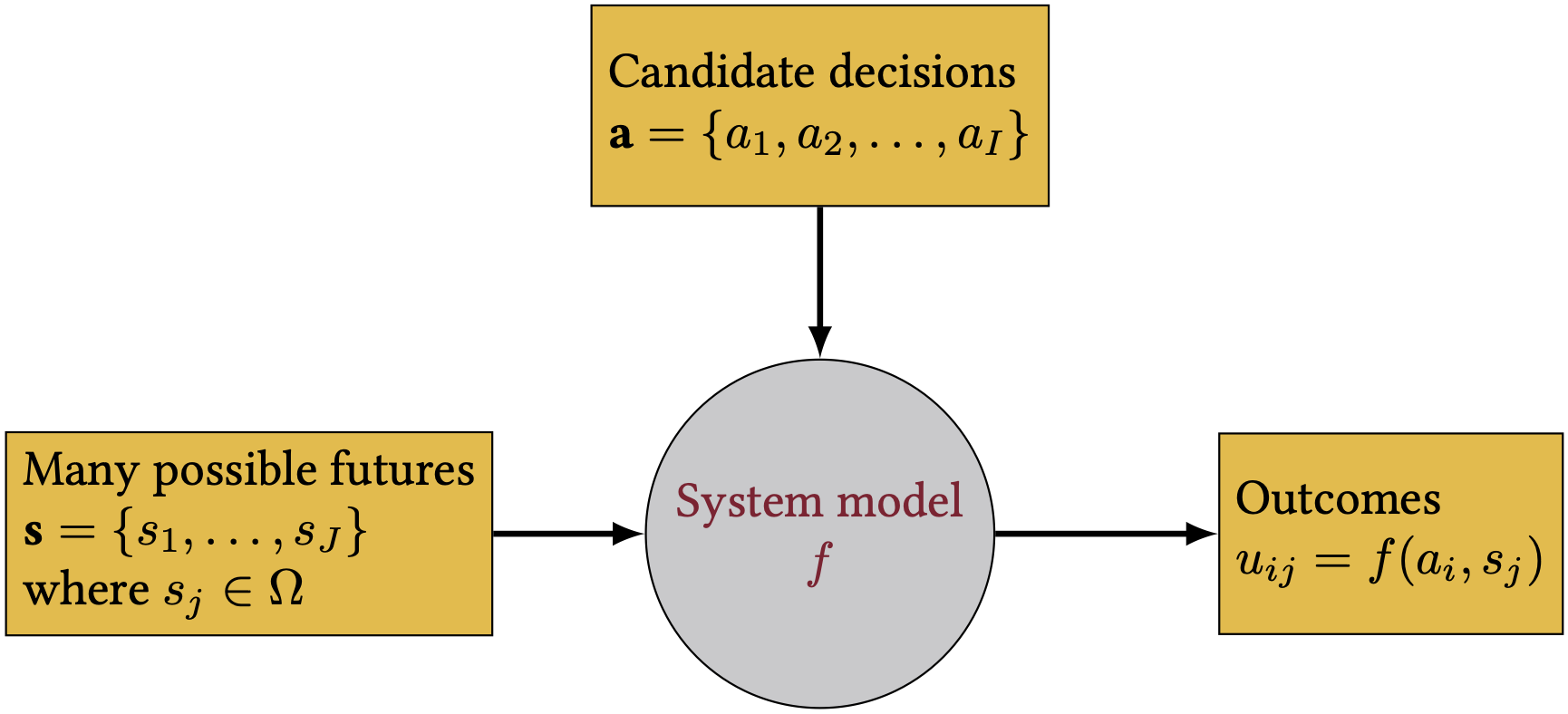
van Dantzig used optimization to inform an engineering design decision. Let’s formalize the general framework.
Optimization Fundamentals
Every optimization problem has the same mathematical structure:
van Dantzig averaged over flood uncertainty analytically. More generally, when the objective or constraints depend on uncertain quantities \(\boldsymbol{\theta}\):
