Global Sensitivity Analysis

Lecture

Dr. James Doss-Gollin

Wednesday, February 25, 2026

Draft: This content is under development.

Reading

• Sensitivity Analysis: The Basics from Reed et al. (2022)
• Pianosi et al. (2016)
• Saltelli et al. (2008)

Two Questions About Uncertainty

• VOI: Which uncertainty, if resolved, would most change my decision?
• GSA: Which uncertainty contributes most to the variability in my output?

These are not the same question, and the answers can disagree.

“We just covered VOI. Now I want to introduce a complementary tool.” Write both questions in different colors. “A parameter can dominate the output variance but have zero EVPI — if it doesn’t change which action is best.”

What Is Sensitivity Analysis?

SA investigates how variation in a model’s output is attributed to variation in its inputs (Pianosi et al., 2016).

\[Y = g(X_1, X_2, \ldots, X_M)\]

• Which inputs cause the largest variation in \(Y\)?
• Are there inputs whose variability has negligible effect?
• Are there interactions between inputs?

“We have a model — could be your dike model, a climate model, an economic model. It takes uncertain inputs and produces an output. SA asks: which inputs matter?”

Three Purposes of SA

1. Screening (factor fixing): which inputs can I safely ignore?
2. Ranking (factor prioritization): which input matters most?
3. Mapping: what input combinations produce extreme outputs?

Typical workflow: screen → rank → map.

“Start cheap — screening tells you which inputs to throw out. Then rank the rest. Mapping is the most expensive but most useful for decision-making.” “For your final project, you’ll want to do at least ranking.”

Local Sensitivity: One-at-a-Time

Vary one input at a baseline \(\bar{\mathbf{x}}\), hold all others fixed:

\[ S_i^{\text{local}} \approx \frac{\partial g}{\partial x_i} \bigg|_{\mathbf{x} = \bar{\mathbf{x}}} \]

Approximate with a finite difference (\(M + 1\) evaluations):

\[ \hat{S}_i = \frac{g(\bar{x}_1, \ldots, \bar{x}_i + \Delta_i, \ldots) - g(\bar{\mathbf{x}})}{\Delta_i} \]

“You’ve already done this — in Lab 5 you ran RCP 8.5, then RCP 2.6. That’s OAT.” “It’s cheap and gives you a quick first look. But it has problems.”

OAT Limitations

• Measures sensitivity at one point — may differ elsewhere
• Misses interactions between parameters
• Baseline choice is arbitrary
• Does not explore the full input range

Ask: “What’s the problem with changing one thing at a time?” Sketch 2D input space: SLR on one axis, discount rate on the other. OAT only explores the cross through the center. Global SA fills the whole square.

Going Global

Global SA varies all inputs simultaneously across their full ranges.

• Captures the full range of each input
• Detects nonlinear effects
• Captures interactions between inputs

Two representative methods: Morris (OAT from many starting points) and Sobol indices (variance decomposition).

“Global doesn’t mean you can’t do OAT. Morris does OAT from many random starting points. The key is covering the full input space, not just one baseline.”

The Morris Method (Elementary Effects)

Repeat the local finite difference from \(r\) random starting points. For each input \(i\) and trajectory \(j\):

\[ EE_i^j = \frac{g(\ldots, \bar{x}_i^j + \Delta_i, \ldots) - g(\ldots, \bar{x}_i^j, \ldots)}{\Delta_i} \]

Summarize across trajectories:

• Mean of \(|EE_i|\): overall influence (ranking)
• Std. dev. of \(EE_i\): interactions or nonlinearity

Cost: \(r(M+1)\) evaluations (e.g., \(10 \times 6 = 60\) for \(M = 5\)).

“Morris is just the local calculation repeated from many different starting points. Then you look at how the sensitivity changes across the input space.”

Reading a Morris Plot

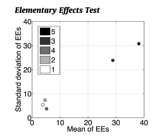
Figure 1: Source: Pianosi et al. (2016), Appendix A.

• Near origin: unimportant — screen out
• Far right, low SD: strong main effect
• Far right, high SD: important and interactive

“This one plot tells you everything. Near the origin — doesn’t matter, throw it out. Far right — it matters. If the SD is also high, it’s interacting with other inputs.”

Variance Decomposition

For independent inputs, the total variance decomposes:

\[ \text{Var}(Y) = \sum_i V_i + \sum_{i<j} V_{ij} + \cdots + V_{12\ldots M} \]

• \(V_i = \text{Var}\bigl(\mathbb{E}[Y \mid X_i]\bigr)\): main effect of \(X_i\)
• \(V_{ij}\): interaction between \(X_i\) and \(X_j\)
• Higher-order terms exist but are rarely important in practice

“The total variance of the output splits into pieces: how much comes from each input alone, how much from pairs interacting, and so on. In practice, first-order and second-order terms capture nearly everything. You’ll rarely see higher-order interactions reported in the literature.”

Sobol Indices

First-order — if you knew \(X_i\), what fraction of the variance in \(Y\) would go away?

\[ S_i = \frac{\text{Var}\bigl(\mathbb{E}[Y \mid X_i]\bigr)}{\text{Var}(Y)} \]

Total-order — if you knew everything except \(X_i\), what fraction of the variance would remain?

\[ S_{T_i} = 1 - \frac{\text{Var}\bigl(\mathbb{E}[Y \mid X_{\sim i}]\bigr)}{\text{Var}(Y)} \]

where \(X_{\sim i}\) denotes all inputs except \(X_i\).

“\(S_i\): if you could pin down this one input, how much would your uncertainty in the output shrink? That’s the main effect. \(S_{T_i}\): if you pinned down everything else, how much uncertainty would be left? That captures the input’s main effect plus all its interactions. If \(S_i \approx S_{T_i}\) for every input, the model is approximately additive — no interactions.” Go slowly — this is the most notation-heavy part.

Interpreting Sobol Indices

Pattern	Interpretation
\(S_i\) large, \(S_{T_i} \approx S_i\)	Strong main effect, few interactions
\(S_i\) small, \(S_{T_i}\) large	Matters mainly through interactions
\(S_i\) small, \(S_{T_i}\) small	Doesn’t matter much
\(\sum S_i \approx 1\)	Model is mostly additive

Screening rule: \(S_{T_i} \approx 0\) is necessary and sufficient for unimportance (Pianosi et al., 2016).

“This table is your cheat sheet for reading Sobol indices.” Walk through each row with a concrete example from the dike problem.

Reading a Sensitivity Analysis

Three questions to always ask:

1. What inputs were varied? Different scope → different results
2. What distributions were assumed? Change the distribution, change the indices
3. Are the results converged? Finite samples give estimates, not exact values

“If someone hands you a sensitivity analysis — or you’re doing one yourself — this is your checklist.”

The Distribution Assumption

Every GSA calculation requires a probability distribution \(p(X_1, \ldots, X_M)\).

\(\text{Uniform}(-\pi, \pi)\) gives different Sobol indices than \(\text{Normal}(0, 0.1)\).

“The definition of the input variability space is one of the most delicate steps in the application of GSA.” — Pianosi et al. (2016)

“This is the punchline, and it connects back to VOI. Both VOI and GSA require probability distributions over the inputs. When you can’t specify those distributions confidently — that’s deep uncertainty. That’s Week 8.”

Summary

• VOI: which uncertainty affects the decision?
• GSA: which uncertainty affects the output?
• These are not the same — answers can disagree
• Both require probability distributions over inputs
• When you can’t specify distributions → deep uncertainty (Week 8)

“Two complementary tools, same requirement. Next week we break that requirement.” “Friday’s lab puts VOI to work on the dike problem from Lab 5.”

References

Pianosi, F., Beven, K., Freer, J., Hall, J. W., Rougier, J., Stephenson, D. B., & Wagener, T. (2016). Sensitivity analysis of environmental models: A systematic review with practical workflow. Environmental Modelling & Software, 79, 214–232. https://doi.org/10/f8n6zw

Reed, P. M., Hadjimichael, A., Malek, K., Karimi, T., Vernon, C. R., Srikrishnan, V., et al. (2022). Addressing uncertainty in multisector dynamics research. Zenodo. Retrieved from https://doi.org/10.5281/zenodo.6110623

Saltelli, A., Ratto, M., Andres, T., Campolongo, F., Cariboni, J., Gatelli, D., et al. (2008). Global sensitivity analysis: The primer. John Wiley & Sons, Ltd. Retrieved from http://onlinelibrary.wiley.com/doi/abs/10.1002/9780470725184.ch1