Exploratory Modeling & Scenario Discovery

Lecture

James Doss-Gollin

Monday, March 23, 2026

From Lab 7: What Drove Failure?

So far you have three tools for analyzing decisions under uncertainty:

• GSA (Week 7): which inputs explain the most variance in outcomes?
• Value of Information (Week 8): would learning more change your decision?
• Robustness (Week 8): how well does a policy hold up across scenarios?

Today: which conditions in that ensemble actually drove failure?

Target: 1:03. “What drives failure?” is fundamentally different from “what’s the best policy?” — it doesn’t require aggregating over scenarios.

Uncertainty in Simulation Models

Srikrishnan et al. (2022) distinguish three sources of uncertainty in coupled human-natural systems:

• Parametric uncertainty: we know the model structure, but not the exact parameter values
  Example: climate sensitivity, damage function coefficients
  This is the target of Monte Carlo sampling and GSA (Weeks 4, 7).

• Structural uncertainty: we don’t agree on which equations represent the system
  Example: ice sheet dynamics, damage function form, discount rate model
  Requires running multiple model structures — a multi-model ensemble.

• Sampling uncertainty: finite samples from stochastic processes
  Example: 30 years of storm surge records from a non-stationary climate
  Addressable with more data or better sampling designs, but never fully eliminated.

Target: 1:06. Parametric = what we’ve been sampling (MC, GSA). Structural = harder, requires multi-model ensembles. When both are large → deep uncertainty → need exploratory modeling.

Defining uncertainty

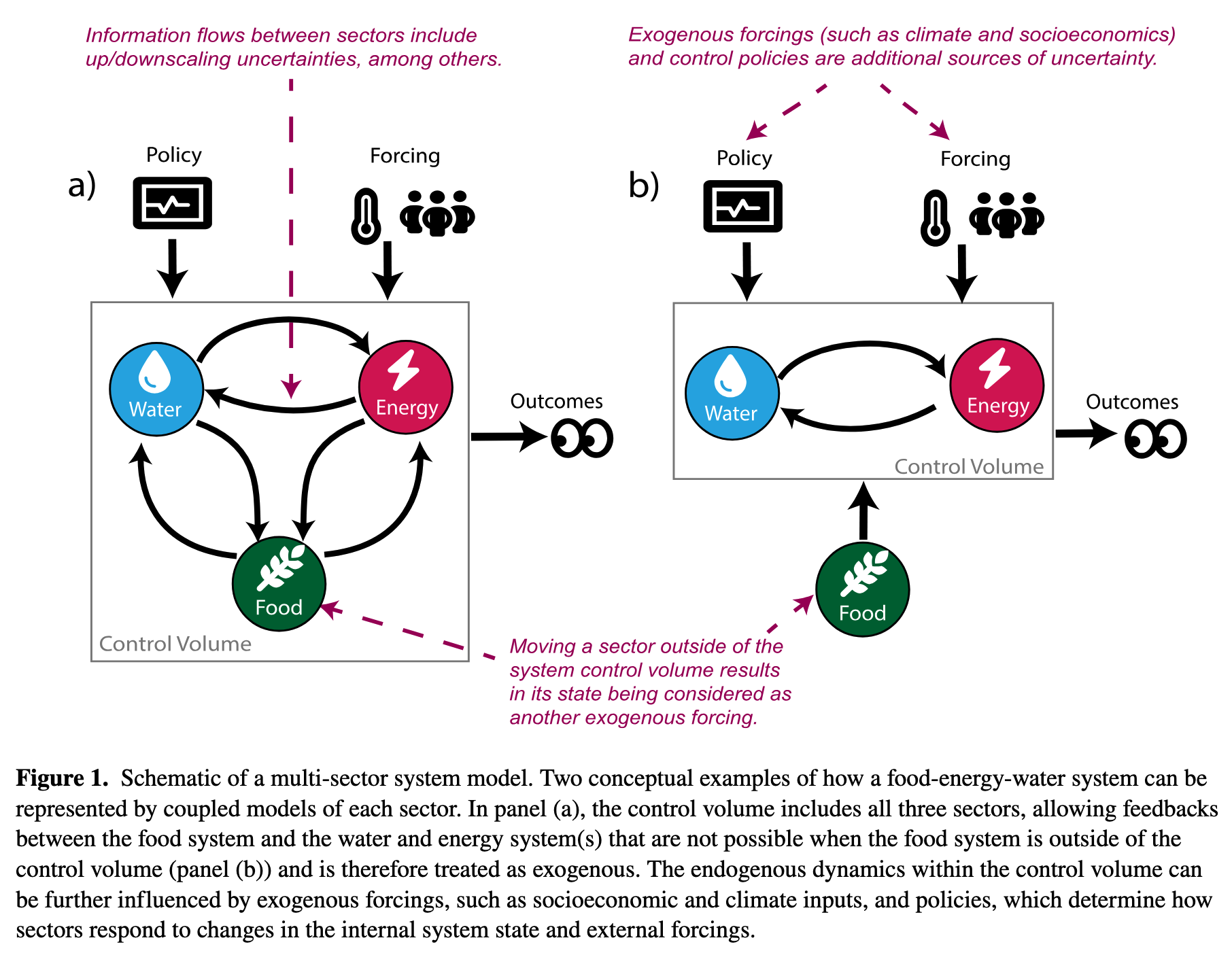
Figure 1: Srikrishnan et al. (2022)

Target: 1:08.

Exploratory Modeling

Today

1. Exploratory Modeling

2. Scenario Discovery

Target: 1:08.

Consolidative vs. Exploratory Modeling

Bankes (1993) identifies two fundamentally different uses of simulation models:

Consolidative modeling

• Synthesize all available knowledge into one best model
• Use it to predict outcomes
• Works when you can validate the model against data over the relevant horizon

Examples: calibrated GCMs for physical climate projection, structural engineering load analysis, tidal prediction

Exploratory modeling

• Use computation to systematically explore the space of plausible models and assumptions
• Each run is a computational experiment probing one corner of the assumption space

Examples: century-scale climate adaptation, integrated assessment of climate policy

The key criterion: can you validate the model? For decadal-to-century scale socio-environmental systems, the answer is usually no.

Target: 1:14. Key pushback response: “Can you validate a 2100 SLR projection? No. So what do we do with those models?” Not admitting defeat — using computation for what it’s good at: exploring a large space systematically.

Discussion: When Is Consolidative Modeling Enough?

Think-Pair-Share (90 seconds)

Give two examples of problems where a consolidative model is appropriate, and one where it is not. What distinguishes them?

Target: 1:17. 60s think, 30s pair, cold-call 2-3. Consolidative: weather (< 10 days), bridge loads, orbits. Exploratory: 50-year flood risk, pandemic policy, energy transitions. Distinguishing factor: can you validate on the relevant timescale?

What Exploratory Modeling Requires

Running thousands of scenarios across uncertain parameters and policy choices:

\[(\mathbf{X}, \mathbf{L}) \xrightarrow{\mathbf{R}} \mathbf{M}\]

• X: uncertain inputs — varied across their plausible range
• L: policy levers — varied to compare strategies
• R: system model — the simulation being run
• M: metrics — the outcomes we track

A large ensemble maps the outcome space: how metrics vary across the full space of assumptions and decisions.

Target: 1:19. Key distinction from standard MC: exploratory modeling varies X and L simultaneously — “what happens under different policies AND different futures?”

Scenario Discovery

Today

1. Exploratory Modeling

2. Scenario Discovery

Target: 1:20.

The Scenario Discovery Workflow

1. Define one or many policies to evaluate
   e.g., elevate house by 1 meter; or compare 0.5m, 1m, 1.5m elevations
2. Run the model across a large ensemble: \(N\) draws of uncertain inputs \(\mathbf{X}\)
3. Label each run: success (\(y=0\)) or failure (\(y=1\)) based on a metric threshold
4. Classify: find which regions of \(\mathbf{X}\)-space concentrate failures
5. Interpret: translate the classification into narrative scenarios

Sometimes we want to find what breaks a single policy. Sometimes we want to compare which scenarios break different policies.

Target: 1:23. Step 3 is a value judgment — the failure threshold is the analyst’s choice. Lab 8 implements all five steps. Multi-policy example: Lamontagne et al. vary the policy lever alongside uncertainties.

How Do We Classify? A Spectrum of Methods

Three common approaches, each with different tradeoffs:

Method	Strength	Weakness
Logistic regression	Familiar; interpretable coefficients; probabilistic output	Assumes linear decision boundary
CART	Visual; handles interactions; no linearity assumption	Can overfit; splits can be unstable
PRIM	Designed for scenario discovery; coverage/density tradeoff	Less familiar; requires tuning

The right choice depends on the problem — interpretability often matters more than classification accuracy.

Target: 1:25. Lab 8 uses PRIM. Today: logistic regression via Lamontagne, then PRIM.

CART: Recursive Splitting

CART partitions the input space by recursive binary splits. At each node, find the variable \(X_k\) and threshold \(t\) that minimizes Gini impurity in the two resulting child nodes:

\[G_m = 2\, p_m\,(1 - p_m)\]

where \(p_m\) is the fraction of failures in node \(m\) (\(G_m = 0\) is pure; \(G_m = 0.5\) is maximally mixed).

\[\text{Best split: } \underset{X_k,\, t}{\arg\min}\; \frac{N_L}{N} G_L + \frac{N_R}{N} G_R\]

Why minimize Gini? Each split should make the children as pure as possible — nodes where almost all scenarios are failures, or almost none are.

Target: 1:28. Greedy algorithm — locally optimal splits, not globally optimal. This is why trees can be unstable. Gini penalizes impurity quadratically: 50/50 is much worse than 70/30, driving the algorithm to find the most informative splits first.

CART vs. Random Forests

A single CART tree is a deterministic partition: one tree, one set of rules.

A random forest builds hundreds of trees, each on a random subsample of the data and features, then averages their predictions.

• Random forests are more accurate and more stable
• But the output is a black box — you can’t read off simple “if/then” rules
• For scenario discovery, we want interpretable boundaries, not maximum accuracy

Discussion

Why might a decision-maker prefer a single, less accurate tree over a more accurate but opaque ensemble?

Target: 1:31. 30s think, then 2-3 responses. Key answer: communicability. “Fails when SLR > X and discount rate < Y” can go in a report. A forest gives a probability but no simple explanation.

CART: From Tree to Partition

Each leaf predicts the majority class — failure (\(y=1\)) if more than half its scenarios are failures.

Example: a two-level tree on SLR rate and flood damage might produce:

Leaf	SLR (m/century)	Flood Damage ($B)	Majority
1	\(\leq 0.5\)	any	success
2	\(> 0.5\)	\(\leq 2\)	success
3	\(> 0.5\)	\(> 2\)	failure

Result: interpretable “if/then” rules — but boundaries are fixed top-down, not iteratively refined.

Target: 1:33. Same geometry as PRIM boxes, but CART splits top-down while PRIM peels from outside in. Draw the 2D partition on the board if time allows.

Think-Pair-Share: Labeling Failures

Scenario

A city is evaluating a coastal sea wall sized for a 1-in-50-year storm surge, at a cost of $200M. Uncertain inputs: storm surge magnitude, sea level rise rate, future population exposure, discount rate, construction cost overrun.

Write (90 seconds)

In one sentence, define what “failure” means for this decision. Then write which two inputs you expect most drive failures and why.

Pair: Compare with your neighbor. Did you define failure the same way?

Target: 1:35. 90s write, 60s pairs, cold-call 2-3. Key point: failure definition is a value judgment — different definitions → different scenario discovery results. Their intuition may be wrong; that’s what SD is for.

Logistic Regression: The Model

For scenario \(i\) with input vector \(\mathbf{z}_i\), model the log-odds of failure:

\[\log \frac{p_i}{1 - p_i} = b_0 + b_1 z_{i1} + b_2 z_{i2} + \cdots = \mathbf{b}^\top \mathbf{z}_i\]

Solving for \(p_i\) gives the sigmoid function:

\[p_i = \frac{1}{1 + e^{-\mathbf{b}^\top \mathbf{z}_i}}\]

\(p_i \in (0, 1)\) always. Classify as failure if \(p_i \geq 0.5\), which is equivalent to \(\mathbf{b}^\top \mathbf{z}_i \geq 0\).

Target: 1:37. Not predicting which scenario is “likely” — asking: given this combination of inputs, what’s the probability of failure? Key limitation: decision boundary is a hyperplane (flat). Failures in a corner of input space require interaction terms.

Interpreting Logistic Regression

The quantity \(\log \frac{p}{1-p}\) is the log-odds — the logarithm of the odds of failure. A fitted coefficient \(b_k\) tells you: a one-unit increase in \(X_k\) shifts the log-odds by \(b_k\).

The odds ratio \(e^{b_k}\) gives a multiplicative interpretation:

“A one-unit increase in \(X_k\) multiplies the odds of failure by \(e^{b_k}\).”

Example: if \(b_k = 0.7\), then \(e^{0.7} \approx 2\) — a unit increase in \(X_k\) doubles the odds of failure.

Rank inputs by \(|b_k|\) (after standardizing) to answer: which inputs most drive failure?

Target: 1:40. Connection to GSA: Sobol indices rank by variance explained; logistic regression ranks by log-odds and gives direction (positive/negative).

Lamontagne et al. (2019): The Setup

Lamontagne et al. (2019) ask: what abatement pathways lead to tolerable climate/economic futures, given deep uncertainty about human-Earth system (HES) dynamics?

Model: DICE integrated assessment model (climate + economy coupled)

Ensemble: 5,200,000 scenarios — 24 HES uncertain parameters + abatement growth rate (\(\alpha\))

Failure label: “intolerable” if warming \(> 2^\circ\)C in 2100, OR abatement cost \(> 3\%\) of GWP, OR climate damages \(> 2\%\) of GWP

Their methodology combines two tools you already know:

1. Sobol sensitivity analysis (Week 7) to rank the 24 uncertain parameters by importance — identifying which factors explain the most variance
2. Logistic regression (scenario discovery) to map how failure probability varies across the dominant factors — identifying where in the input space failure concentrates

Target: 1:42. GSA and scenario discovery complement each other: GSA tells you which factors matter, SD tells you where things go wrong. Wednesday digs into the figures.

Lamontagne et al. (2019): The Finding

After labeling 5.2M runs as tolerable/intolerable, logistic regression on the dominant inputs shows:

The primary control on 2100 warming is the abatement growth rate — a societal choice, not an exogenous physical uncertainty.

Near-term warming is controlled by climate sensitivity (a physical parameter). Long-term warming is controlled by earlier abatement actions (a policy choice).

It is mostly a question of whether we choose to limit warming — not whether we can.

Wednesday we will dig into the figures: how the Sobol indices shift over time (Fig 2), and what the logistic regression contours look like (Fig 3).

Target: 1:44. Near-term warming is locked in (physics); long-term depends on what we do now. SD gives you “what drives outcomes,” not “what will happen.” For Wednesday: why do time-varying Sobol indices (Fig 2b-d) tell a different story than time-aggregated (Fig 2a)?

PRIM: Patient Rule Induction Method

PRIM finds a box in the input space that concentrates failures:

\[a_k \leq X_k \leq b_k \quad \text{for each input } k\]

Interpretation: “The strategy fails when SLR \(> 0.8\,\text{m}\) AND storm surge return period \(< 25\,\text{years}\)” is a PRIM box in two dimensions.

“Patient” refers to the algorithm: PRIM peels small slices from the box one at a time. Each peel removes the thinnest slice with the fewest failures.

Target: 1:46. Box = axis-aligned rectangle. Key design choice: interpretability — communicable to non-technical audiences. “Patient” contrasts with CART’s larger splits. Students implement PRIM in Lab 8.

PRIM: Coverage and Density

For a box \(B\) over an ensemble with \(N\) total runs, \(N_f\) of which are failures:

\[\text{Coverage} = \frac{|\{\text{failures inside } B\}|}{N_f} \qquad \text{(recall)}\]

What fraction of all failures does the box capture?

\[\text{Density} = \frac{|\{\text{failures inside } B\}|}{|\{\text{scenarios inside } B\}|} \qquad \text{(precision)}\]

Of all scenarios in the box, what fraction are failures?

Target: 1:47. Coverage = recall. Density = precision. Full space → coverage 1, density = base rate. Tiny box → density ~1, low coverage.

The Coverage–Density Trade-off

PRIM starts with the full input space and peels away small slices to increase density, recording coverage as it goes.

The output is a peeling trajectory: a set of nested boxes tracing the Pareto frontier in coverage–density space.

• Start: large box, high coverage, low density
• Peel: remove slices where failures are sparse
• End: small box, high density, low coverage
• The analyst chooses the box that best matches their decision context

Target: 1:48. Analogy: fishing net. Large net = high coverage, lots of bycatch. Fine mesh = high density, small haul. Safety-critical → prefer coverage. Communication → prefer density. Knee-point usually works well.

Write-and-Respond: Interpreting a PRIM Box

PRIM analysis of a 1-meter house elevation policy returns:

Box	SLR Rate (m/century)	Storm Return Period	Coverage	Density
A	\(> 0.4\)	any	94%	31%
B	\(> 0.8\)	\(< 25\) yr	71%	82%
C	\(> 1.1\)	\(< 10\) yr	34%	96%

Write (60 seconds)

In one sentence, interpret Box B. Then answer: if you are advising a city that faces severe storm surge risk and deep uncertainty in SLR, which box would you recommend and why?

Target: 1:49. 60s write, 3-4 responses. Box A: high coverage, low density. Box B: good balance. Box C: very specific, misses most failures. No “right” answer — the choice depends on values and context.

Friday’s Lab: The Eijgenraam Dike Model

In Lab 8 you’ll apply scenario discovery to a real flood protection problem from the Netherlands (Eijgenraam et al., 2014).

You know the Van Dantzig problem: how high should we build the dike? Eijgenraam extends it — investment costs grow exponentially with height, and flood risk grows over time with sea level rise and economic growth. (Rhodium example)

The decision: when to heighten the dike and by how much.

• Deferring saves money (discounting) but the dike ring is unprotected while we wait
• Building higher is safer but exponentially more expensive

Target: 1:50. Preview only — keep conceptual, math is on next slide.

The Eijgenraam Model: Key Equation

The annual flood probability at year \(t\) is:

\[P(t) = P_0 \exp\bigl(\alpha \eta\, t - \alpha\, H(t)\bigr)\]

• \(P_0\): initial flood probability
• \(\alpha\): sensitivity of flood probability to water level (1/cm)
• \(\eta\): rate of water level rise (cm/year)
• \(H(t)\): cumulative dike heightening at time \(t\)

This assumes an exponential distribution for water levels — analytically convenient, though real flood distributions have heavier tails.

Notice: \(\alpha\) appears twice — it makes risk grow faster (\(\alpha \eta t\)) and makes each cm of dike more effective (\(-\alpha H\)). Its effect on failure is non-monotonic.

Target: 1:50. High alpha → more sensitive to water level (bad for risk growth, good for dike effectiveness). Students will discover this through PRIM on Friday.

Lab 8: The XLRM Setup

XLRM	Lab 8
X (uncertainties)	\(P_0\), \(\alpha\), \(\eta\), \(V_0\), \(\delta\)
L (levers)	\((T_{\text{heighten}},\; \Delta H)\) — when to heighten, how much
R (model)	Eijgenraam cost-benefit model
M (metrics)	Max failure probability, total cost

Your task: fix a policy, run 1,000 scenarios, label success/failure, and use PRIM to find which uncertainties drive failure.

The twist: changing how you define failure changes which uncertainties matter.

Target: 1:50. Don’t spoil the twist — let them discover that changing the failure definition changes which uncertainties matter.

Looking Ahead

Wednesday: Figure discussion of Lamontagne et al. (2019)

Friday: Lab 8 — Scenario Discovery on the Eijgenraam dike model + Memo 1 due

Target: 1:50. Memo 1 reminder: students should have a complete XLRM diagram and narrative.

Figure Discussion Sign-Up

Wednesday’s discussion: each person leads a 3-minute walkthrough of one figure from Lamontagne et al. (2019).

Slot	Figure(s)	Focus
1	Fig 1a	Sampling the policy space
2	Fig 1b–d	Tradeoff clouds & “tolerable” windows
3	Fig 2a	Time-aggregated Sobol sensitivities
4	Fig 2b–d	Time-varying sensitivities
5	Fig 3a–b	Robust pathways at low climate sensitivity
6	Fig 3c + conclusion	Median sensitivity & headline message

Sign up now!

Target: 1:50. Take names verbally. Each person also preps one discussion question. < 6 students: combine slots 5+6. > 6: split Fig 2b-d into individual panels.

References

Bankes, S. (1993). Exploratory modeling for policy analysis. Operations Research, 41(3), 435–449. https://doi.org/10/c7rgcr

Eijgenraam, C., Kind, J., Bak, C., Brekelmans, R., den Hertog, D., Duits, M., et al. (2014). Economically efficient standards to protect the Netherlands against flooding. INFORMS Journal on Applied Analytics, 44(1), 7–21. https://doi.org/10.1287/inte.2013.0721

Lamontagne, J. R., Reed, P. M., Marangoni, G., Keller, K., & Garner, G. G. (2019). Robust abatement pathways to tolerable climate futures require immediate global action. Nature Climate Change, 9(4), 290–294. https://doi.org/10.1038/s41558-019-0426-8

Srikrishnan, V., Lafferty, D. C., Wong, T. E., Lamontagne, J. R., Quinn, J. D., Sharma, S., et al. (2022). Uncertainty analysis in multi-sector systems: Considerations for risk analysis, projection, and planning for complex systems. Earth’s Future, 10(8), e2021EF002644. https://doi.org/10.1029/2021EF002644