Sequential Decision Making

Lecture

James Doss-Gollin

Monday, March 30, 2026

Three Infrastructure Puzzles

• The Tagus River bridge (Lisbon, 1966) was built for road traffic. Rail was added in 1999 — because the original design reserved the option.

• A satellite constellation (de Weck et al., 2004): staging deployment in phases rather than launching all satellites at once improved expected value by ~30%.

• A parking garage in England reinforced its columns during construction. Extra floors were added later when demand grew.

What do these have in common?

Target: 1:03. All three embedded flexibility deliberately — at a cost — before the future was known. The Tagus bridge story is especially nice: the engineers in 1966 couldn’t know if rail would ever be built, but they kept the option alive. The satellite example shows this isn’t just civil infrastructure — staged deployment is a general principle. Ask students: “What’s the cost of building in this flexibility?” — It’s paid upfront, regardless of whether the option is exercised.

Real Options: Vocabulary

A real option is the right — but not the obligation — to take an action in the future.

• Option premium: upfront cost to preserve flexibility Reinforcing the columns; over-engineering the bridge

• Option value: expected gain from having the option Higher expected NPV (ENPV), lower downside risk

• You exercise the option only when conditions favor it — asymmetric upside

Options are valuable precisely because the future is uncertain. If you knew the future, you’d either always build the extra floors or never.

Target: 1:06. The asymmetry point is key: you only exercise when good, so bad outcomes don’t cost you the extra investment. This will connect naturally to the formal framework — a real option IS a policy with a rule.

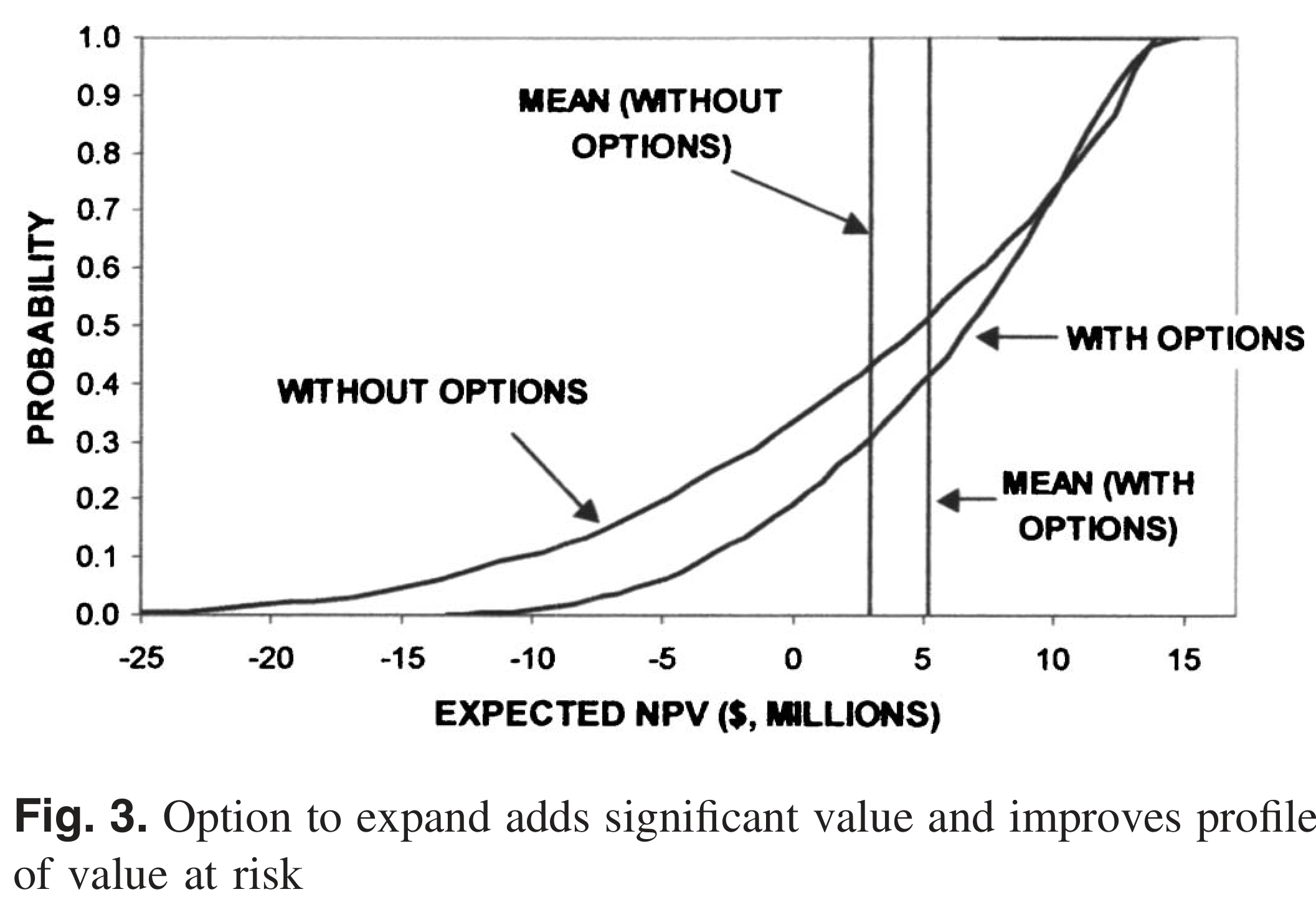
The Parking Garage

de Neufville et al. (2006) — paper you’ll discuss Wednesday.

Design choice: 4 floors with strong columns (option to expand) vs. 6 floors rigid

	No flexibility	Flexible
Initial cost	$22.7M	$14.5M
Expected NPV	$2.87M	$5.12M
Minimum NPV	−$24.7M	−$12.6M
Maximum NPV	$13.8M	$14.8M

Option value ≈ $2.25M — the flexible design wins on ENPV, minimum NPV, and initial cost.

de Neufville et al. (2006)

Target: 1:10. Walk through the table. The flexible design actually costs LESS upfront (build 4 floors, not 6) AND has higher ENPV. The columns cost extra, but you avoid the cost of over-building. The VaR figure makes the asymmetry vivid: the rigid design has a long left tail; the flexible design truncates it. Don’t over-explain — they’ll go deep on Wednesday. Just establish the pattern.

From Static to Sequential

So far in this course: choose one action \(a^*\) today, commit.

\[a^* = \arg\min_{a \in \mathcal{A}} \; \mathbb{E}\!\left[\text{Cost}(a, \mathbf{s})\right]\]

This ignores two things we know to be true:

1. We learn over time — SLR observations will sharpen; storm records will grow.
2. Actions have lifetimes — a dike built to 3.5m today constrains what you can do in 2040.

Sequential decision making asks: what rule should govern each future choice, given what you observe at the time you choose?

Target: 1:13. Make the transition crisp. This is the pivot from Module 2 to today. “Rule” is the key word — we’re not picking an action, we’re picking a mapping from observations to actions.

Two Paradigms for Planning Under Uncertainty

Herman et al. (2020) classifies decision support frameworks for water resources planning under climate change into two families:

Herman et al. (2020)

Target: 1:15. Robust planning (Weeks 7–9): find alternatives that hold up across scenarios. Bottom-up, scenario-based. Students know this well. Dynamic planning (today): design policies that respond to new observations over time. Higher dependence on uncertainty characterization because you’re optimizing a sequence of decisions through time, not just a single action. A dynamic plan can also be robust; static robust plans tend toward overdesign because they can’t exploit information as it arrives. Point to the figure: dynamic planning is highlighted. Note that both can co-exist in practice.

The Control Problem: Components

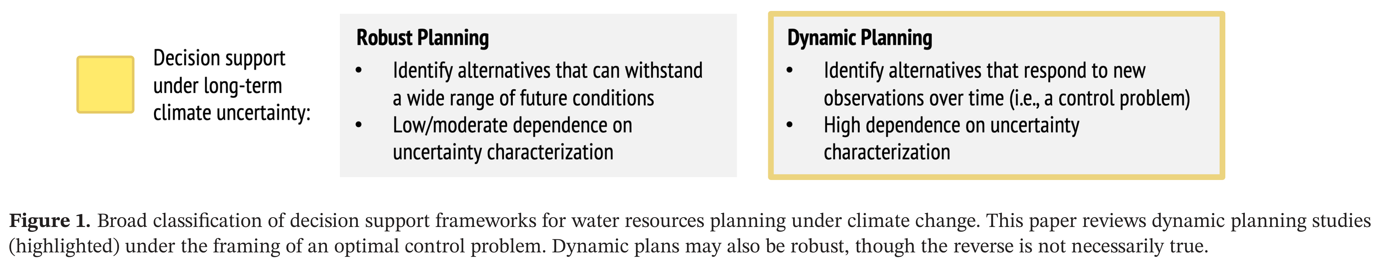
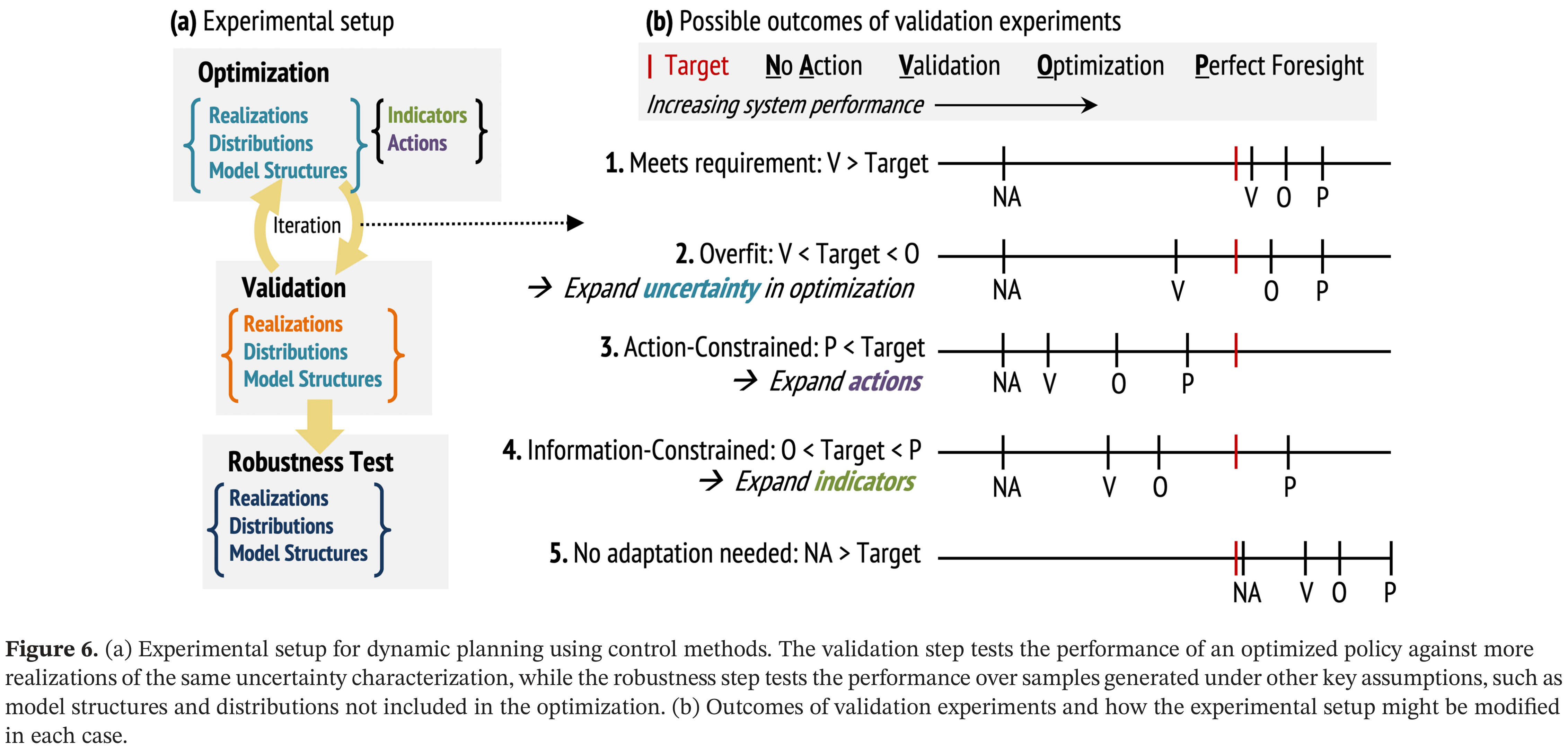
Dynamic planning has four components: policy structure, uncertainty characterization, solution method, and validation.

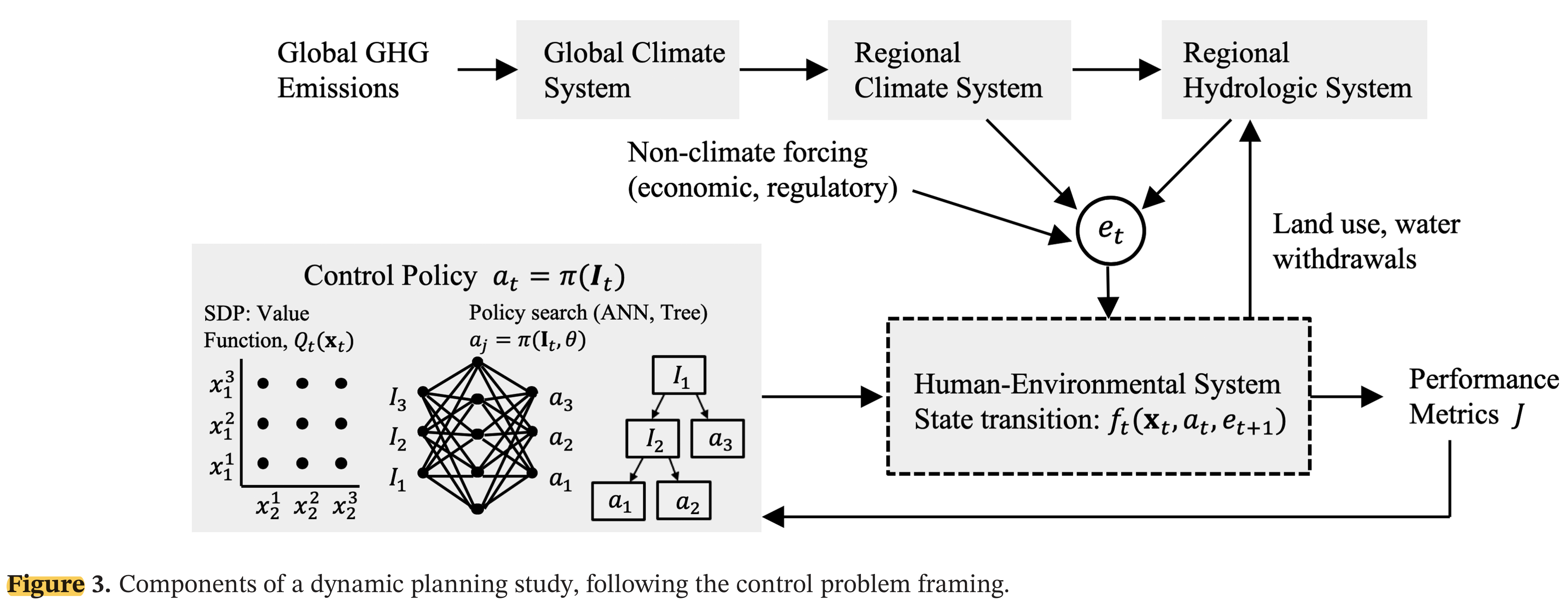
The control policy \(\pi\) (left box) observes the system and selects actions \(a_t\). Forcing \(\mathbf{e}_t\) propagates through the climate-hydrology chain into the human-environmental system, producing performance metrics \(J\). From Herman et al. (2020).

Target: 1:17. Walk students through the diagram carefully — this is the conceptual map for the lecture. Left box: the policy. Two flavors shown — SDP (value function Q, discretized states) and policy search (ANN or tree mapping I_t to a_t). We’ll discuss both. Top: the chain of forcing uncertainty — GHG emissions → GCM → regional climate → hydrology. This is the “cascade of uncertainty” from Herman. Center: the human-environmental system with its state transition f_t. This is where dike heights, reservoir levels, and infrastructure capacity live. Right: performance metrics J — cost, damages, reliability. The non-climate forcing arrow (economic, regulatory) is a nice reminder that human systems are also uncertain.

State, Action, Forcing

Formal setup: at each time step \(t\),

Symbol	Meaning	Example
\(\mathbf{x}_t\)	System state	Dike height, reservoir storage
\(a_t \in \mathcal{A}\)	Action	Heighten by \(u_t\); expand; do nothing
\(\mathbf{e}_t\)	Stochastic forcing	SLR realization, storm surge, precipitation
\(J_t\)	Cost	Investment cost + expected damages

State transition: \(\mathbf{x}_{t+1} = f_t(\mathbf{x}_t,\; a_t,\; \mathbf{e}_{t+1})\)

Convention: actions are chosen after observing \(\mathbf{x}_t\)

Target: 1:20. Walk through the table one row at a time. “The dike height is a state — it’s a number we observe before we decide. The forcing is stochastic — we don’t know next year’s storm surge, but we do know the dike height right now.” The state transition equation: given where we are, what we do, and what happens, where do we end up?

Policy and Objective

The agent applies a policy \(\pi\) to observable information \(\mathbf{I}_t\):

\[a_t = \pi(\mathbf{I}_t)\]

\(\mathbf{I}_t\) can include current states, trend estimates, projections — anything observable.

Objective: minimize expected total cost over a planning horizon \(H\):

\[\min_\pi \; \mathbb{E}_{\mathbf{e}}\!\left[\sum_{t=0}^{H-1} J_t(\mathbf{x}_t,\; a_t,\; \mathbf{e}_{t+1})\right]\]

We are optimizing a rule, not a sequence of actions. Solution methods specify how to find the best \(\pi\)

Target: 1:23. Dwell on the distinction: optimizing a rule vs. optimizing actions. In the static case, we pick numbers (dike height = 3.5m). In the sequential case, we pick a function (“raise the dike when the observed water level exceeds the buffer by X cm”). The expectation is over all the uncertainty in forcing — this connects to scenarios they’ve been using all semester. The subscript on the expectation, E_e, is important: we’re averaging over possible forcing trajectories. Each trajectory is a scenario. The last line sets up the three solution methods to follow.

Why Is This Hard? Three Sources of Uncertainty

Herman et al. (2020) identify three distinct sources:

1. Sampling uncertainty — finite historical record; rare events underrepresented. 30 years of storm surge data doesn’t capture the full tail.

2. Exogenous hydroclimate uncertainty — cascade from emissions → GCMs → downscaling → hydrology. Dynamic changes (precipitation, storm tracks) far more uncertain than thermodynamic (SLR, snowpack).

3. Endogenous human-environment uncertainty — water demand, land use, institutional capacity. Often exceeds climate uncertainty on decadal planning horizons.

Similar to Srikrishnan et al. (2022) framing, more tailored to water resources.

A policy optimized against a narrow set of scenarios may fail outside that envelope.

Target: 1:27. This taxonomy is directly from the paper. It’s useful because different uncertainty types call for different responses. Key insight: thermodynamic changes (SLR, snowpack loss) are more detectable and plannable around than dynamic changes (precipitation trends). That affects what indicator variables are useful. The last line is critical — foreshadows the validation discussion at the end.

Solution Method 1: Open-Loop Control

The simplest approach: decide the full action sequence now, commit.

\[\{a_0,\; a_1,\; \ldots,\; a_{H-1}\} = \pi(t)\]

Actions depend only on time, not on observations.

• Optimize once, then execute
• No feedback — same dike-heightening schedule regardless of whether SLR is fast or slow
• Computationally simple; 300-year problem = 300 decision variables

Target: 1:30. This is what the Garner/Keller “intertemporal” formulation does — 300 annual heightenings decided at the start. Students can intuit the problem: if you set a schedule in 2025 assuming median SLR, you’ll under-build in the high-SLR future and over-build in the low-SLR future. The policy can’t adapt.

Solution Method 2: Stochastic Dynamic Programming

Closed-loop: work backward from the terminal state using Bellman’s equation.

\[Q_t(\mathbf{x}_t) = \min_{a_t} \; \mathbb{E}_{\mathbf{e}_{t+1}}\!\left[\; J(\mathbf{x}_t,\; a_t,\; \mathbf{e}_{t+1})\; +\; \gamma\, Q_{t+1}(\mathbf{x}_{t+1})\; \right]\]

• \(Q_t(\mathbf{x})\): optimal cost-to-go from state \(\mathbf{x}\) at time \(t\)
• Recursive: solve \(Q_H\), then \(Q_{H-1}\), …, then \(Q_0\)
• The expectation requires a probability model for \(\mathbf{e}_{t+1}\) — you must encode all uncertainty into the transition distribution
• Curse of dimensionality: computational cost explodes with the number of state variables

Target: 1:34. The Bellman equation: “Today’s optimal action depends on the expected value of being in each possible future state, weighted by how likely each future state is.” Emphasize the key constraint: SDP requires you to specify a probability distribution for the forcing, AND to discretize the state space. If your uncertainty is deep — if you can’t write down a credible probability model — SDP struggles. Curse of dimensionality: doubling the number of state variables squares the state space. Practical limit is about 3-4 continuous state variables.

Solution Method 3: Direct Policy Search

Instead of solving for the value function, parameterize the policy directly:

\[a_t = \pi(\mathbf{I}_t,\; \theta)\]

\(\theta\) can parameterize a threshold rule, a radial basis function, a neural network — any differentiable or simulable function.

Optimize \(\theta\) by evaluating the policy over an ensemble of scenarios:

\[\min_\theta \; \frac{1}{N}\sum_{i=1}^{N} \sum_{t=0}^{H-1} J_t^{(i)}(\mathbf{x}_t,\; \pi(\mathbf{I}_t,\; \theta),\; \mathbf{e}_{t+1}^{(i)})\]

where \(i\) indexes scenarios.

Target: 1:38. This is the key insight to land hard. In SDP, you encode uncertainty into a probability model inside the equation. In DPS, you draw scenarios and simulate. Students have been drawing scenarios and simulating since Week 4. Function classes for π: simple threshold rules, radial basis functions, neural networks. The choice is a modeling decision. DPS scales much better than SDP: 10 parameters instead of a full value function over a discretized state space. Optimizer: often an evolutionary algorithm (can handle non-smooth, high-dimensional θ search).

DPS in Action: The Levee Problem

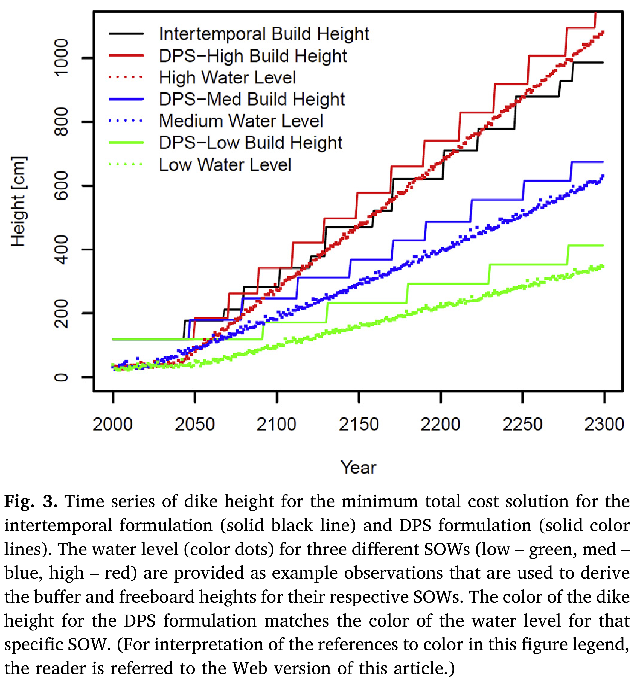
• Intertemporal (open-loop): prescribe annual heightenings \(u_1, \ldots, u_{300}\) at the start. Same schedule for every future.
• DPS (closed-loop): observe the rate of water rise and variability around the trend. Apply a rule: “heighten by enough to restore the buffer, plus freeboard.”

Garner & Keller (2018)

Target: 1:41. The figure makes the idea vivid without requiring students to have read the paper. Key observation: the intertemporal policy is a single rigid staircase — same for every scenario. The DPS policy adapts: under the high-SLR scenario (red) it builds aggressively; under the low-SLR scenario (green) it barely builds at all. Result: DPS achieves lower cost AND lower damages — it dominates the intertemporal approach. Save the detailed mechanics (what exactly the state variables are, the Pareto comparison) for Wednesday’s discussion.

Choosing Indicator Variables

The policy \(\pi(\mathbf{I}_t, \theta)\) is only as useful as the information in \(\mathbf{I}_t\).

• An indicator = variable + timescale + aggregation window + transform “30-year moving average of annual inflow” “Rate of water rise over the prior 30 simulation years”

• False positive: adapt when you didn’t need to — wasted investment

• False negative: fail to adapt when you should — damages or failure

• Short observation window → more false positives

• Long observation window → more false negatives

Thermodynamic signals (SLR, snowpack) detectable sooner. Dynamic signals (precipitation trends) may take 50+ years to emerge.

Target: 1:44. The false positive / false negative framing connects to frequentist hypothesis testing students know from statistics. The thermodynamic vs. dynamic distinction from Herman: sea level is a cleaner signal than precipitation. This affects what you should be watching. We’ll revisit indicator selection more carefully next week with case studies.

Real Options Revisited

Now that we have the vocabulary: a real option is simply a policy with a rule.

The parking garage policy:

\[a_t = \begin{cases} \text{add a floor} & \text{if occupancy} > \tau \text{ for two consecutive years} \\ \text{do nothing} & \text{otherwise} \end{cases}\]

This is \(\pi(\mathbf{I}_t, \theta)\) with \(\theta = \tau\) and \(\mathbf{I}_t = \text{occupancy}_t\).

De Neufville found it by intuition and simulation. DPS finds it by optimization over \(\theta\) across many scenarios.

The option premium = cost of reinforcing the columns = cost to make this policy feasible.

Target: 1:46. This is the payoff of the opening. The connection should feel satisfying — we’ve been building toward this since slide 1. “Building in the real option” = choosing a state transition function \(f\) that makes certain future actions possible. You can only build the extra floors if the columns were reinforced.

Evaluating vs. Designing Policies

These are different tasks and are easy to confuse.

Evaluating a policy: given fixed \(\theta\), simulate over scenarios and compute costs. This is what robustness analysis in Weeks 7–8 did.

Designing a policy: search over \(\theta\) to minimize expected costs across the ensemble. This is what DPS does.

The quality of a designed policy depends on the quality of the uncertainty characterization used during optimization.

Target: 1:48. The distinction matters practically: a policy evaluated robustly may still have been designed against a narrow set of scenarios. If the future is outside that envelope, the policy may fail.

Validation: How Good Is Your Policy?

Test the optimized policy against scenarios not used in optimization.

Herman et al. (2020)

Target: 1:49. Five possible outcomes for a policy tested out-of-sample: 1. Meets requirement — good 2. Overfit — performs well in training, not in validation; need more/different scenarios 3. Action-constrained — even perfect foresight can’t meet target; need different actions 4. Information-constrained — perfect foresight works but your policy doesn’t; need better indicator variables 5. No adaptation needed — target met without doing anything; maybe you already have enough robustness The distinction between cases 3 and 4 is especially useful: it tells you whether you need to change WHAT you can do vs. WHAT you observe.

Summary

• Real options: build in the right to act later; option value = ENPV gain from flexibility
• Sequential decisions: optimize a policy \(\pi(\mathbf{I}_t, \theta)\) — a rule mapping observations to actions
• Open loop: no feedback; must over-build to cover worst case
• SDP: closed loop, exact, requires probability model + discretized state space
• DPS: closed loop, scalable, evaluates policy over scenarios — the framework we’ve been using
• Validation: evaluating ≠ designing; test out-of-sample or risk overfit to your training scenarios

Wednesday: Fuad leads discussion of de Neufville et al. (2006).

Target: 1:50. The summary list should feel like a coherent arc, not a bag of concepts.

References

References slide — no notes needed.

Garner, G. G., & Keller, K. (2018). Using direct policy search to identify robust strategies in adapting to uncertain sea-level rise and storm surge. Environmental Modelling & Software, 107, 96–104. https://doi.org/10.1016/j.envsoft.2018.05.006

Herman, J. D., Quinn, J. D., Steinschneider, S., Giuliani, M., & Fletcher, S. (2020). Climate adaptation as a control problem: Review and perspectives on dynamic water resources planning under uncertainty. Water Resources Research, e24389. https://doi.org/10.1029/2019wr025502

de Neufville, R., Scholtes, S., & Wang, T. (2006). Real Options by Spreadsheet: Parking Garage Case Example. Journal of Infrastructure Systems, 12(2), 107–111. https://doi.org/10.1061/(asce)1076-0342(2006)12:2(107)

Srikrishnan, V., Lafferty, D. C., Wong, T. E., Lamontagne, J. R., Quinn, J. D., Sharma, S., et al. (2022). Uncertainty analysis in multi-sector systems: Considerations for risk analysis, projection, and planning for complex systems. Earth’s Future, 10(8), e2021EF002644. https://doi.org/10.1029/2021EF002644