Sequential Decision Problems
Lecture
This lecture borrows heavily from Herman et al. (2020).
Introduction
House elevation problem
Thus far, we have looked at a single static decision: how high to elevate the house. However, in many cases, decisions are not static, but rather sequential. For example, we don’t necessarily need to make this decision today! Instead, we could wait and see how fast local sea-levels are rising, and then make a decision later with more information.
General dynamic decision problems
Dynamic planning problems identify policies to select actions in response to new information over time. Policy design involves choosing the sequence, timing, and/or threshold of actions to achieve a desired outcome. This typically involves a combination of optimal control and adaptive design.
Optimal control and reinforcement learning
Optimal control and reinforcement learning are related fields relating to the study of optimizing sequential decision problems.
For a thorough but accessible textbook on reinforcement learning, I recommend Sutton & Barto (2018).
Framing
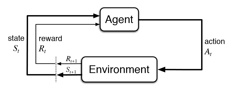
In sequential decision problems, the decision maker does not need to make all decisions at once. Instead, at each time step, the decision maker makes a decision based on the state of the system (which may not be fully observable). In our case study, the state might include the current elevation of the house, the current sea level, and other potential variables.
Mathematically, the state evolves over time according to a dynamics model, which describes how the state changes in response to the decision maker’s actions and external factors: \[ \mathbf{x}_{t+1} = f_t(\mathbf{x}_t, a_t, e_{t+1}), \] where
- \(\mathbf{x}_t\) is the state at time \(t\)
- \(a_t\) is the decision at time \(t\) (e.g. whether we elevate and if so how high)
- \(e_{t+1}\) is some forcing (e.g., the rate of sea level rise)
- \(f_t\) is assumed deterministic, but it can evolve over time.
Reward
A key concept in sequential decision problems is that at each time step, the decision maker gets some immediate feedback. This is often called reward, \(R\). The reward \(R_{t+1}\) (indices by convention) depends on the state at time \(t\), the action at time \(t\), and the forcing at time \(t\).
In our house elevation problem, the reward might be the cost of flood insurance and the cost of elevating (which will often be zero).
Policy
The decision maker’s strategy for choosing actions is called a policy. The policy is a deterministic (or stochastic) function that maps states to actions. We’ll focus here on discrete time problems, although continuous time problems are also well-studied in some domains.
Expected future rewards
A central idea of optimal control problems is to maximize the expected sum of future rewards.1 The basic idea is that there might be actions that give a low reward now, but that lead to high rewards in the future. In our case study, an illustration would be spending a lot of money to elevate the house now, but then not having to pay as much for flood insurance in the future. Future rewards are usually discounted (as we have seen); this can be done either in the cost function or in the reward function.
This leads naturally to an important concept in reinforcement learning: value. The value of a state is the expected sum of future rewards that can be obtained from that state, assuming the decision maker follows a particular policy. The value of a state-action pair is the expected sum of future rewards that can be obtained from that state, assuming the decision maker takes a particular action and then follows a particular policy.
Solution methods
There are many methods for solving sequential decision problems! Here, we’ll focus on a few examples from Herman et al. (2020). This is not by any means a comprehensive list.
On Wednesday we’ll read a paper that compares what we call here open loop (they call it “intertemporal open loop control”) and dynamic policy search.
Open loop
Open loop control solves for all actions at once. The result is a vector of actions corresponding to each time step.
The primary advantage of open loop control is that it’s very easy to execute the policy – no further analysis, updating, or optimization is needed. The primary disadvantage is that it’s not adaptive – it doesn’t take into account new information that might be available later. It can also be computationally challenging because it requires solving a lot of decision variables (each time step is a decision variable) and they are not independent (if I elevate my house in 2030, I probably don’t want to elevate it in 2031).
Dynamic programming
There are many variations of dynamic programming, but the most commonly applied is stochastic dynamic programming, in which the value function \(Q\) for each state at time \(t\) is estimated from the recursive Bellman equation: \[ Q_t(\mathbf{x}_t) = \min_{a_t} \left\{ R_t + \gamma Q_{t+1} (\mathbf{x}_{t+1}) \right\}. \] where \(\gamma\) is the discount factor.
This problem is typically discretized and solved using a backward induction algorithm. In other words, a discrete number of states and actions are considered. The discrete state transition function gives you the probability of transitioning from one state to another, given an action. A very rough solution approach is:
- Calculate the value function for the each step in last time step, \(Q_T(x^1_T), Q_T(x^2_T), \ldots\).
- For each time step \(t = T-1, T-2, \ldots, 1\), calculate the value function for each state \(x_t\) using the Bellman equation:
- For each state \(x_t\), calculate the value of each action \(a_t\) as the reward plus the discounted expected value of the next state
- Choose the action that maximizes the value function
- The value function for the state is the value of the action that maximizes the value function
An advantage of methods like SDP is that they can provide exact solutions to the problem, conditional on the model and discretization. A disadvantage is that often very strong assumptions are required to discretize the problem and make it tractable. SDP also suffers from the “curse of dimensionality” because as the number of states and actions increases, the number of possible state-action pairs increases exponentially.
Policy search
Policy search assumes a specific functional form for a policy \(\pi\) with parameters \(\theta\) such that \(a_t = f(\mathbf{x}_t, \theta)\). The goal is to find the parameters \(\theta\) that maximize the expected sum of future rewards.
Common choices of \(f\) include linear decision rules, radial basis functions, binary trees, and neural networks. A primary advantage of policy search is that it can be very flexible and adaptive, and can be used with simulation-optimization frameworks. A primary disadvantage is that it can be computationally expensive and can require a lot of data to estimate the parameters.
In our case study, there are many different ways to parameterize our decision rule. Two options suggested by (garnergarner_slrise:2018?) are:
- define a “buffer height” as the minimum tolerable elevation of the house relative to the mean sea level and a “freeboard height” so that when the buffer height is exceeded, the house is elevated to be BH + FH above the mean sea level.
- Estimate FH and BH based on the local slope and acceleration of the sea-level
However, very complex control rules using deep neural networks are also used (e.g., in video game playing).
Discussion
Like everything we’ve seen in this class, we are using a model to represent the real world, but the model isn’t the real world and we should take this into account when designing and interpreting our optimization.
Flexibility
The financial theory of real options defines “the right, but not obligation” to take a particular action in the future. For example, if I purchase the right to buy Apple stocks in 1 year at price \(X\), I can choose to buy the stocks if the price is higher than \(X\), but I don’t have to buy them if the price is lower than \(X\). This is a real option, and it has value.
This has motivated study of options in engineering and policy design. It turns out that creating flexibility in decision making can be very valuable, but it’s not always easy to generate designs that are naturally flexible. An example we’ll see on Friday gives a simple example: build a parking garage to a few floors, build it to many floors, or build a few floors but extra-strong so we can add levels in the future if needed? (Neufville et al., 2006).